Four Stage Reproducible Time Series Anomaly Detection for Researchers

Anomaly detection in time series works best as a four-stage pipeline: preprocess with detrending and STL decomposition, detect with statistical baselines before reaching for machine learning, score the output, then post-process before anyone acts on it. Start with STL plus residual rules, roughly the tsoutliers approach. Escalate to forecasting or reconstruction models only when seasonality gets complex or the data is multivariate.
TL;DR:
- Classical statistical methods are most effective for series with clear seasonality and normal noise, especially when running on sparse or short datasets.
- Deep learning models, such as LSTM and autoencoders, are justified mainly when dealing with irregular seasonality, complex variable relationships, or shape-based anomalies.
- Proper pipeline stages—preprocessing, detection, scoring, and post-processing—are essential to reduce false positives and improve detection reliability.
- Synthetic benchmarks may overstate the effectiveness of complex models, so real- and event-level evaluation with time tolerance remains the most honest assessment.
- Reproducibility and clear explanation of flagged anomalies are critical, with statistical methods offering more transparent and explainable outputs than deep learning approaches.
Table of Contents
- What Types of Anomalies Show Up in Time Series?
- What Is the Standard Pipeline for Detecting Anomalies?
- Which Statistical Methods Should You Try First?
- When Do You Need Machine Learning or Deep Learning Models?
- Which Tools Should You Actually Use?
- How Do You Evaluate and Benchmark a Detector Honestly?
- What Mistakes Do Most TSAD Projects Make?
- How Does PlotStudio Support Research-Grade TSAD Experiments?
- How Do You Handle Multivariate Time Series Anomaly Detection?
- What Changes When Detection Has to Run in Real Time?
- Can You Actually Explain Why a Model Flagged Something?
- When Should You Prioritize Rigor Over Speed?
- Build Reproducible Anomaly Detection Pipelines With PlotStudio
- Sources
What Types of Anomalies Show Up in Time Series?
Not every spike is the same kind of problem, and the type dictates which detector actually works.
- Point anomalies are single observations that break from their neighbors, like a sensor reading that jumps for one timestamp and returns to normal. Statistical rules and simple thresholds catch these well.
- Contextual anomalies look normal in isolation but wrong given the surrounding context, such as a retail spike that’s fine on Black Friday but alarming on a random Tuesday. Seasonal decomposition handles these because it separates the calendar-aware baseline from the raw value.
- Collective or subsequence anomalies are short segments where no single point looks unusual, but the shape of the segment does, like a heart rate that stays technically in range while its rhythm goes erratic. Reconstruction and representation-based methods are built for this.
- Whole-series anomalies flag an entire series as unusual relative to a population of similar series, which is a clustering or distance problem, not a pointwise one.
One trap catches almost everyone eventually: a sustained shift isn’t an anomaly, it’s a regime change. If a metric permanently moves to a new baseline after a policy change or system upgrade, the fix is re-fitting your model to the new regime, not tuning your detector to catch it as an outlier every time.
What Is the Standard Pipeline for Detecting Anomalies?
A decade-spanning survey of the field converges on a process-centric taxonomy that splits every time series anomaly detection method into four stages, and that framing holds up whether you’re running a statistical rule or a deep model.
- Preprocessing. Validate the data, resample to a consistent frequency, and decide how to handle missing values, since gaps distort both trend and seasonal estimates. Apply detrending and STL seasonal adjustment here, not later. Skipping this step is the single most common reason detectors flag “anomalies” that are just uncorrected seasonal cycles.
- Detection. The core model, statistical, forecasting-based, reconstruction-based, or distance-based, produces a raw signal indicating how unusual each point or window is.
- Scoring. Convert that raw signal into a comparable score, then set a threshold. Fixed thresholds are simple but brittle; percentile-based or IQR-based thresholds adapt better across series with different variance.
- Post-processing. Group adjacent flagged points into single events, smooth noisy scores, and route ambiguous cases to a human reviewer before anything downstream (an alert, a retraining trigger) fires automatically.
That last stage gets skipped more than any other, and it’s usually why teams end up drowning in false alarms within a month of deployment.
Which Statistical Methods Should You Try First?
Classical methods remain the right starting point for most anomaly detection time series work, not because they’re simpler, but because they’re auditable, fast, and often just as accurate.
The standard workflow starts with STL (or MSTL for multiple seasonal periods) decomposition, splitting the series into trend, seasonal, and remainder components. Rob Hyndman’s approach to this, run the outlier check on the remainder, not the raw series, since the remainder isolates what the trend and seasonal terms can’t explain.
Statistic: When STL remainders are approximately normally distributed, Tukey’s 3×IQR rule flags an extremely low proportion of normal points as “far out” when residuals are approximately normally distributed. This results in an extremely low false-positive rate for a rule this simple.
That single fact explains why so many production monitoring systems still lean on decomposition plus IQR thresholds instead of a neural network: the math is transparent, the false-positive behavior is well understood, and you can explain a flagged point to a stakeholder in one sentence.
- STL + remainder-based IQR: best for series with clear seasonality and roughly normal noise.
- Control charts (Shewhart, CUSUM): strong for process-monitoring contexts where drift matters as much as spikes.
- ARIMA with automatic outlier detection: the tsoutliers workflow fits an ARIMA model, locates additive outliers, level shifts, and temporary changes, removes them, refits, and iterates until nothing significant remains. It’s particularly useful when outliers are biasing your forecast model’s parameter estimates, not just cluttering a dashboard.
Classical methods tend to win outright on sparse data, noisy-but-seasonal data, and any series short enough that a deep model has nothing meaningful to learn from. Save the heavier machinery for when the signal genuinely needs it. For a deeper look at distributional assumptions behind these thresholds, see outlier detection methods.
When Do You Need Machine Learning or Deep Learning Models?
Escalate past statistical baselines when seasonality is irregular, the relationship between variables matters, or the anomaly is a shape, not a value. Three model families dominate this space.
- Forecasting-based models predict the next value and score anomalies by prediction error. LSTM and Seq2Seq architectures handle nonlinear temporal dependencies that ARIMA can’t, and Transformer-based predictors are increasingly common when the series has long-range dependencies. The scoring logic is straightforward: large, persistent prediction error signals an anomaly, small error is noise.
- Reconstruction-based models, autoencoders, variational autoencoders, and GANs, learn to reconstruct normal patterns and flag points the model reconstructs poorly. These assume the training data is mostly normal, which matters because a reconstruction model trained on contaminated data learns to reconstruct the contamination too.
- Representation and distance-based methods cluster series or subsequences and flag points far from any cluster center. Micro-clustering approaches in the spirit of MCOD are built specifically for subsequence and whole-series anomalies where pointwise scoring fails outright.
Deep learning models handle multivariate temporal and spatial structure better than traditional methods when the data actually supports that complexity, which is the real justification for reaching for PyTorch and an LSTM instead of stopping at STL.
Labeled anomalies are almost always scarce, which is why semi-supervised and self-supervised training strategies, training a forecaster or autoencoder only on data assumed normal, tend to outperform fully supervised classifiers in practice. You don’t need thousands of labeled anomalies; you need a clean baseline period.
Pro Tip: Calibrate your anomaly threshold on a held-out window you’re confident is anomaly-free, not on the same window you used to train the model. A threshold that looks great on training data usually collapses the first week it sees production traffic.
For guidance on choosing between forecasting architectures for error-based scoring, forecasting accuracy covers model selection tradeoffs that apply directly here.
Which Tools Should You Actually Use?
Mapping methods to libraries is where most guides get vague. Here’s the concrete version.
- ADTK handles rule-based and seasonal detectors with a unified API, and its pipe classes let you compose transformers and detectors into a single reproducible object. It’s the fastest path from “I have a hunch” to a working seasonal detector, and its built-in NYC taxi dataset example is a solid template for a first pipeline.
- statsmodels implements STL and MSTL decomposition directly, which covers the preprocessing stage of nearly every pipeline in this article. For time series analysis methods beyond decomposition, statsmodels also handles the ARIMA fitting that feeds into a tsoutliers-style workflow.
- scikit-learn covers clustering-based detection and gives you IsolationForest as a fast, dependency-light baseline before you commit to anything heavier.
- PyTorch is where you build custom LSTM forecasters or autoencoders once statistical baselines stop being enough. The official LSTM documentation is the right starting reference for sequence length, hidden state sizing, and batching conventions.
- tsoutliers ® remains the cleanest implementation of automatic ARIMA-based outlier detection, locating additive outliers, level shifts, and temporary changes, then iterating until the model is clean.
None of these tools replace good judgment about which method category fits your anomaly type. They just make the implementation reproducible, which matters more than most teams admit until a reviewer asks how a result was produced. For code generation workflows that keep this reproducible end to end, see Python code generation.
How Do You Evaluate and Benchmark a Detector Honestly?
Event-level evaluation with time-tolerant matching, crediting a detection if it falls within a reasonable window of the true event, is the more honest metric, paired with precision, recall, and PR AUC rather than plain accuracy.
Note: Benchmarking work presented at NeurIPS found that classical algorithms can outperform recent deep learning approaches on properly matched synthetic and real datasets, which is a strong argument against assuming a deep model is automatically stronger.
- Use behavior-driven synthetic datasets to stress-test specific failure modes, but treat their assumptions skeptically. Synthetic anomalies are often too clean compared to what real sensors and systems produce.
- Validate on at least one labeled real dataset alongside synthetic ones. Evaluation design, not just model choice, often decides which method looks best.
- Use rolling or blocked time-aware cross-validation, never a random shuffle split, since a random split leaks future information into training and inflates every metric you report.
- Report threshold sensitivity explicitly. A detector that only works at one exact threshold is not a robust detector.
What Mistakes Do Most TSAD Projects Make?
The same handful of mistakes show up across nearly every failed deployment, and all are avoidable.
- Skipping detrending and seasonal adjustment, then wondering why the detector flags every holiday and every Monday.
- Deploying a black-box model before establishing a simple, interpretable baseline to compare against.
- Setting thresholds on training data instead of a held-out, ideally anomaly-free, validation window.
- Shipping without a feedback loop, so flagged events never get reviewed, grouped, or fed back into recalibration.
Pro Tip: Plot the STL remainder before you do anything else. If it still shows an obvious visual pattern, your detector will find “anomalies” that are really just leftover seasonality you failed to remove.
How Does PlotStudio Support Research-Grade TSAD Experiments?
Sensitive time series data, patient monitoring streams, clinical trial telemetry, financial records under regulatory review, often can’t leave the researcher’s machine at all. Plotstudio runs analysis locally, which makes it workable for IRB-governed or GDPR special-category data that a cloud tool simply can’t touch.
Every anomaly detection pipeline runs behind an analysis plan you approve before code executes, capturing your chosen thresholds and detection method as a pre-registration record. Skills let a lab encode its own detection conventions once and reuse them, and every run exports as an annotated notebook and PDF report a reviewer can trace start to finish.
How Do You Handle Multivariate Time Series Anomaly Detection?
Multivariate anomaly detection time series problems fail the moment you treat correlated metrics as independent series. A server that shows normal CPU and normal memory separately might still be anomalous because the relationship between the two has broken, high memory with unusually low CPU, for instance, which no univariate detector will ever catch.
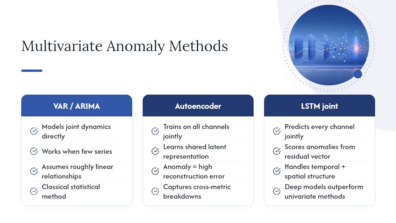
Three approaches handle this reasonably well. Vector autoregression and multivariate extensions of ARIMA model the joint dynamics directly, which works when the number of series is small and their relationships are roughly linear. Autoencoders trained across all channels simultaneously learn a shared latent representation, and reconstruction error spikes when the cross-metric relationship, not any single value, breaks down. LSTM-based forecasters extended to multivariate inputs predict every channel jointly and score anomalies from the combined residual vector, which is where deep models genuinely outperform classical ones, since handling inter-metric spatial structure alongside temporal structure is exactly what traditional univariate methods can’t do.
The practical catch is dimensionality. As the number of monitored series grows, spurious correlations grow with it, and a model trained on 200 loosely related metrics will find “relationships” that are pure noise. Dimensionality reduction, PCA or a learned embedding, before feeding a detector is often what separates a usable multivariate system from a noisy one. Start with the smallest, most causally justified subset of series you can defend, not every metric your monitoring system happens to collect.
What Changes When Detection Has to Run in Real Time?
Real-time anomaly detection time series systems trade accuracy for latency, and that tradeoff has to be made deliberately, not discovered in production.
Batch pipelines can run a full STL decomposition on the entire history every time. Streaming pipelines can’t; they need incremental or windowed decomposition that updates as new points arrive without reprocessing everything. This is where a lot of otherwise solid statistical methods break down in practice, since STL assumes a reasonably complete window to estimate trend and seasonality, and a five-point streaming buffer doesn’t give it one.
Online detection also has to handle concept drift, where the definition of “normal” shifts gradually over weeks or months. A static threshold calibrated once will drift out of relevance; systems built for streaming use adaptive thresholds or periodic recalibration on a rolling recent window instead. A trading platform tracking tick-level anomalies is a good example of how tight the latency budget can get: a detector that takes ten seconds to flag a price anomaly might be functionally useless for the decision it was meant to support.

Alert fatigue is the other real-time-specific failure mode. A detector tuned for offline analysis will often produce far more flags per day than any human reviewer can triage in a streaming context, so post-processing, event grouping, cooldown periods between repeated alerts on the same metric, matters even more online than it does in batch analysis.
Can You Actually Explain Why a Model Flagged Something?
A flagged point without an explanation is a liability, not a result, especially in any research or compliance context where someone will eventually ask why.
Statistical methods win here almost by default. An STL-based flag comes with a built-in explanation: “the remainder exceeded 3 times the interquartile range,” which is a sentence a non-technical stakeholder can verify. A tsoutliers-style flag goes further, classifying the outlier type, additive, level shift, or temporary change, which tells you not just that something broke but roughly how.
Deep models are harder to explain, and that’s not a minor tradeoff. An autoencoder’s reconstruction error tells you that a point was anomalous, not which input dimension drove the error, unless you decompose the reconstruction loss channel by channel. For multivariate LSTM forecasters, per-channel residual contributions serve a similar purpose: they show which of the monitored metrics deviated most rather than presenting a single opaque score.
The practical rule: whatever detector you deploy, make sure its score decomposes into something a domain expert can audit. If it doesn’t, keep a simpler, interpretable baseline running in parallel, not to replace the deep model, but to sanity-check its flags before anyone acts on them.
When Should You Prioritize Rigor Over Speed?
Prototyping fast is fine when you’re exploring whether a signal exists at all. It stops being fine the moment a result feeds a paper, a grant report, or a decision with real consequences. The conversion path is straightforward: lock the analysis plan, document every preprocessing choice, and re-run the final version through a pipeline someone else could reproduce without asking you a single question.
— Aymen
Build Reproducible Anomaly Detection Pipelines With PlotStudio
Every method in this guide, STL decomposition, IQR thresholds, LSTM scoring, still needs a pipeline someone else can audit and rerun, and that’s precisely where most anomaly detection time series work quietly falls apart. Plotstudio runs the entire pipeline locally on your own machine, gates every analysis behind a plan you approve before code executes, and exports an annotated notebook and PDF report that documents exactly how a flagged anomaly was scored.
That matters most for institutions handling patient monitoring data, clinical telemetry, or any dataset an IRB won’t let leave the building; Plotstudio’s local execution is built for exactly that constraint. Skills let your lab define its detection conventions, preferred decomposition method, threshold rule, review steps, once, so every subsequent analysis follows the same auditable process instead of drifting between ad hoc scripts. If your team is running TSAD experiments that need to survive peer review or a compliance audit, explore PlotStudio’s enterprise deployment to see how a research-grade pipeline gets set up for your data.
Sources
- Review describing deep-learning models and their applicability to time series anomaly detection
- Dive into Time-Series Anomaly Detection: A Decade Review
- Anomaly Detection Toolkit (ADTK) documentation