80/20 Causal Inference for Business: Quick Checks, Audit Ready Plans

Causal inference for business estimates what happens because of an action, not what merely correlates with it. When a promotion runs and sales rise the same week, correlation tells you nothing about whether the promotion caused the lift. Businesses turn to randomized experiments when feasible, and to quasi-experimental methods like difference-in-differences, instrumental variables, or Bayesian structural time-series when they aren’t. The rule of thumb: run a formal causal analysis whenever the estimate would change what you actually decide to do.
TL;DR:
- Randomized experiments are ideal but often infeasible; quasi-experimental methods like difference-in-differences or instrumental variables are necessary alternatives.
- DAGs help identify confounders, mediators, and colliders, improving the validity of causal estimates and preventing common adjustment mistakes.
- Bayesian structural time-series models estimate counterfactual trends when no control group exists, but require careful checks like unaffected controls and good pre-intervention fit.
- Proper planning with a detailed Define, Assume, Identify, and Estimate process reduces errors, while operational factors like contamination, sample size, and data quality impact validity.
- Reproducible, plan-first workflows that run locally support compliance, auditability, and transparency, especially with sensitive or regulated data.
Table of Contents
- What Causal Inference Means for Business Decisions
- Experiments and Quasi-Experiments: The Core Method Toolkit
- Bayesian Structural Time-Series: Counterfactuals Without a Control Group
- The Define, Assume, Identify, Estimate Workflow
- Data, Power, and Validation: The Operational Layer
- The Assumption Failures That Quietly Wreck Results
- Building Reproducible, Privacy-Safe Causal Workflows
- Communicating Causal Results Without Losing the Nuance
- Where Causal Inference Runs Into Real Limits
- Software and Packages Analysts Actually Use
- A Reproducible Path From Causal Question to Defensible Result
- Sources
- FAQ
What Causal Inference Means for Business Decisions
Most business dashboards answer predictive questions: what is likely to happen next, given the patterns in historical data. Causal inference answers a different question entirely: what would happen if we intervened? A retention model can predict which customers are likely to churn with high accuracy. It cannot tell you whether sending them a discount code will change that outcome. Only a causal analysis can.
That distinction shows up constantly in marketing, pricing, and product work. A marketing team wants to know the incremental lift of a channel, not just its correlation with revenue during a busy quarter. A pricing team wants to know whether a $2 increase changes unit volume, not whether high-volume periods happen to coincide with lower prices. A product team wants to isolate whether a new onboarding flow improves activation, separate from seasonal traffic swings or a concurrent PR mention.
Causal reasoning formalizes this with the idea of a counterfactual: the outcome that would have occurred under a different action, holding everything else constant. Since you can never observe both the factual and the counterfactual for the same customer at the same time, every causal method is really a strategy for approximating that missing counterfactual. Directed acyclic graphs, or DAGs, help make the reasoning explicit by mapping which variables cause which, and which ones might be quietly distorting your estimate.
DAGs earn their place in a business analyst’s toolkit for a few concrete reasons:
- They force you to name confounders (variables that affect both the treatment and the outcome) before you run any model.
- They expose mediators (variables the treatment works through) so you don’t accidentally strip out the effect you’re trying to measure.
- They flag colliders, a subtler trap covered later, that can create fake associations if you condition on them.
- They document assumptions in a form a stakeholder or reviewer can actually inspect, rather than trusting a black-box output.
Businesses that treat causal modeling as a documented, assumption first exercise catch bad estimates earlier and defend good ones more convincingly.
Experiments and Quasi-Experiments: The Core Method Toolkit
Randomized controlled trials remain the strongest tool available, because random assignment breaks the link between the treatment and any confounder, known or unknown. An A/B test on a checkout flow, a holdout group excluded from a marketing campaign, a geo-randomized pricing test: all share the same logic. Run one long enough to reach the sample size your effect size and baseline conversion rate require, and the result is close to unimpeachable. The catch is feasibility. You can’t randomize a national ad campaign into “on” and “off” for half your customers overnight, and some interventions carry ethical or contractual limits on who can be excluded.
When randomization isn’t available, four quasi-experimental methods cover most business situations:
- Difference-in-differences. Compare the change in an outcome before and after an intervention in a treated group against the same change in a comparable untreated group. This works well for geo-level or market-level rollouts, like launching a feature in one region before others, as long as the two groups would have moved in parallel trends absent the intervention.
- Regression discontinuity. Exploit a hard threshold that assigns treatment, such as a loyalty tier that kicks in above a spend level or a support queue that escalates past a wait-time cutoff. Customers just above and just below the threshold are treated as approximately randomized, which lets you estimate a local causal effect right at that boundary.
- Instrumental variables. Use a variable that affects the outcome only through the treatment, never directly. A classic business example is using regional weather or a supply disruption as an instrument for price changes, since it shifts price without being driven by demand itself. Valid instruments are hard to find, and a weak one produces worse estimates than no instrument at all.
- Bayesian structural time-series (covered in depth below). Build a counterfactual from control time series when neither randomization nor a clean threshold exists.
Choosing among these comes down to three practical questions: Can you randomize without breaking the business or a contract? Do you have a comparable control group with parallel pre-trends? And does a natural threshold or instrument already exist in your data, rather than one you’d have to engineer? Answering those three honestly, before touching a model, saves more analyst time than any statistical trick that comes after.
Bayesian Structural Time-Series: Counterfactuals Without a Control Group
Bayesian structural time-series models solve a specific problem: estimating the effect of an intervention that already happened to everyone, with no held-out group. BSTS trains on a pre-intervention period, using unaffected control series (other markets, related product lines, or correlated external metrics) to predict what the treated series would have done had the intervention never occurred. The gap between that predicted counterfactual and the observed post-intervention data is the estimated causal impact, reported with a posterior credible interval rather than a single point estimate.
Google’s CausalImpact package is the most widely used implementation, and it comes with an explicit set of checks analysts need to run before trusting the output:
- Confirm the control series were genuinely unaffected by the intervention. If a “control” region also saw a marketing spillover, the counterfactual is contaminated.
- Verify pre-period fit quality. A model that fits the pre-intervention data poorly has no business predicting the counterfactual for the post-period.
- Watch the priors, particularly
prior.level.sd. Over-specifying dynamic, time-varying regression terms can overfit and inflate posterior uncertainty rather than sharpen it. - Run a placebo or imaginary intervention test: apply the same model to a period or series where you know nothing happened, and confirm it reports no effect.
Statistic to know: BSTS methodology, as described in the original Google research, produces both pointwise impact estimates and cumulative impact over the full post-period, each with its own credible interval, which is what lets a stakeholder see whether an early spike faded or a lift compounded over weeks.
Synthetic control methods extend the same logic by constructing a weighted combination of untreated units that best mimics the treated unit’s pre-intervention trajectory, often the sharper choice for geo-lift tests where a single market gets a real launch and dozens of others serve as candidate controls. The CausalImpact manual is explicit that skipping the placebo check is the single most common way analysts fool themselves with this class of model.
The Define, Assume, Identify, Estimate Workflow
Most failed causal projects fail before a single line of code runs, because nobody wrote down what question was actually being asked. The four-step causal workflow, Define, Assume, Identify, Estimate, exists to prevent exactly that.
- Define. Write the estimand in plain language: are you estimating the average treatment effect (ATE) across everyone, or the average treatment effect on the treated (ATT), the subgroup that actually received the intervention? State the decision this analysis feeds and what result would change that decision. If a 2% lift and a 6% lift lead to the same choice, you may not need a high-precision estimate at all.
- Assume. Draw the DAG. List every confounder you can measure and, just as important, the ones you can’t. Pre-specify how you’ll adjust for the measured ones before you see the results, not after.
- Identify. Match the estimand to a method that can actually recover it given your assumptions. This is a conceptual step separate from running any model: sometimes the honest answer is that the question isn’t estimable from the data you have, and the right move is to change the question or collect new data, not force an estimator to produce a number anyway.
- Estimate. Run the model, report the effect size alongside a confidence or credible interval, and run robustness checks: alternate specifications, placebo tests, sensitivity to dropped covariates. State the limitations plainly in the same document that states the result.
Pro Tip: Write the Define and Assume steps as a one-page brief before anyone touches data. If a stakeholder can’t agree on the estimand or the DAG up front, no amount of modeling sophistication will make the eventual number persuasive.
Businesses that skip straight to Estimate tend to produce technically defensible numbers that answer the wrong question. A DAG that a Plotstudio causal inference analysis workflow forces you to draw before running code catches that mismatch while it’s still cheap to fix.
Data, Power, and Validation: The Operational Layer
Every causal method above depends on decisions made long before estimation: which metric to trust, how many observations you need, and how to keep the experiment or quasi-experiment clean.
Pick a primary metric that maps directly to the decision, not the metric that’s easiest to compute. Revenue per user beats raw conversion rate when your intervention changes basket size as much as it changes conversion. Define the event window explicitly (does a “conversion” count if it happens three days later through a different channel?) before you collect a single data point, not after you see which definition produces a nicer number.
Sample size and power calculations aren’t optional overhead. A test with too few observations to detect a realistic effect size will report “no significant difference” regardless of whether a real effect exists, which is a different finding than “we proved there’s no effect.” Run a quick power calculation, or a small pilot, before committing budget to a full rollout.
Three operational risks deserve specific attention:
- Contamination between groups. If your test and control audiences overlap through retargeting, shared households, or cross-channel exposure, your effect estimate is biased toward zero.
- Holdout hygiene. A holdout group that quietly shrinks over time, or that support teams accidentally re-include in a campaign, invalidates the comparison without anyone noticing until the results look strange.
- Pre-registration. Writing the analysis plan, primary metric, and success threshold before running the test is the most reliable defense against p-hacking, the practice of testing multiple metrics until one clears significance by chance.
Something worth internalizing: cumulative lift and pointwise lift tell stakeholders different stories, and conflating them is a common source of miscommunication. A campaign that shows a strong pointwise spike in week one but flat pointwise effects afterward can still show a substantial cumulative lift, because the early gains compound. Report both, and label which one supports which claim.
The Assumption Failures That Quietly Wreck Results
Confounding is the most familiar failure mode: an unmeasured variable drives both the treatment and the outcome, creating an association that looks causal but isn’t. DAG-guided adjustment, where you name the confounder and control for it explicitly, reduces this risk, but only for confounders you actually thought to measure.
Collider bias is the trap analysts fall into while trying to be careful. Conditioning on a variable that both the treatment and the outcome influence can create a spurious association where none existed, or hide a real one. A commonly cited example: analyzing only customers who responded to a survey introduces bias if both the treatment and the outcome affect the likelihood of responding.
A few more failure modes worth flagging explicitly:
- Control series in a BSTS or synthetic control analysis that were themselves touched by the intervention, whether through channel spillover or a shared promotional calendar, will bias the counterfactual and hide behind a plausible-looking chart.
- Overfitting a time-series model with too many dynamic regression terms inflates apparent precision without improving actual accuracy.
- Multiple testing across many metrics, regions, or time windows without correction turns a handful of false positives into a “finding” someone will act on.
- External validity gets overstated when a result from one segment, region, or season gets generalized to the whole business without checking whether the mechanism plausibly transfers.
None of these failures are exotic. They’re the default outcome of skipping the Assume step, which is exactly why that step exists in the first place.
Building Reproducible, Privacy-Safe Causal Workflows
A causal estimate that a stakeholder can’t audit is a causal estimate they shouldn’t fully trust, and that’s doubly true once a decision involves real budget or regulated data. Pre-specifying an analysis plan before running any code, then locking in the estimand, assumptions, and success criteria, functions as a pre-registration and an audit trail in one document. That habit, well established in applied research practice, reduces the researcher-degrees-of-freedom problem where an analyst quietly tries several specifications until one looks good.
For teams handling GDPR-governed customer records, IRB-supervised behavioral data, or any dataset that legally can’t leave a controlled environment, local execution isn’t a convenience feature. It’s the difference between being able to run the analysis at all and having to skip it. A workflow where analysis runs on the researcher’s own machine, rather than uploading a customer table to a cloud service, removes that constraint entirely.
Reproducibility closes the loop. Concrete assets worth checking for in any causal workflow, business or academic:
- An analysis plan reviewed and approved before code executes, stating methods and assumptions up front.
- Annotated notebooks that show every transformation applied to the raw data, not just the final chart.
- Exportable PDF reports that a non-technical stakeholder can review without opening a notebook.
- A searchable, permanent record of past analyses, so a supervisor or collaborator can trace exactly how a result three months ago was produced.
Some analysis processes structure their workflows around this sequence, gating execution behind a reviewed plan and keeping data local by default.
Communicating Causal Results Without Losing the Nuance
A confidence or credible interval means nothing to a stakeholder who reads it as a rounding error. The single most useful habit in communicating causal results is stating the range and what decision changes at each end of it, rather than reporting a lone point estimate and letting the audience assume it’s exact. “The campaign lifted revenue by 6%” invites false precision.
Separate the causal claim from everything the causal claim doesn’t cover. An incrementality test can tell you a channel drove real, additional revenue. It can’t tell you whether that revenue was worth the spend, whether the effect will hold next quarter, or whether a different creative would have done better. Business stakeholders often fold all three questions into “did it work,” and an analyst’s job includes gently unbundling them.
Visuals do more work here than tables. A pointwise impact chart with a shaded credible band, next to the cumulative impact chart with its own band, lets a non-technical audience see both the timing and the magnitude of an effect without reading a single number. Pair that with one plain sentence stating the assumption the whole estimate rests on, such as “this assumes the control markets weren’t exposed to the campaign,” so nobody mistakes a conditional estimate for an unconditional fact.

Heterogeneity deserves a mention even when the average effect is the headline number. An average lift of 4% might mean everyone gained 4%, or it might mean one segment gained 15% while another lost 3%. Stating which case applies changes what a stakeholder should do with the finding.
Where Causal Inference Runs Into Real Limits
Causal inference in business settings runs into constraints that academic papers rarely mention. Randomization is often organizationally or contractually impossible: you can’t withhold a legally required disclosure from a control group, and a sales team won’t tolerate an arbitrary discount denial to half its accounts. Quasi-experimental methods fill the gap, but every one of them trades some rigor for feasibility, and that trade needs to be stated, not hidden.
Data quality is a recurring limiter that’s specific to business contexts. Academic datasets are usually collected for the study itself. Business data is a byproduct of operational systems never designed with causal identification in mind, which means missing values, inconsistent event logging across teams, and metric definitions that quietly changed halfway through the period you’re analyzing. A causal estimate is only as trustworthy as the messiest input feeding it.
External validity is another real constraint. An effect measured in one region, one season, or one customer segment doesn’t automatically transfer to another. A pricing elasticity estimated during a holiday period can misrepresent behavior the rest of the year, and a result from your highest-value customer segment may not generalize to the rest of the base at all.
Finally, some causal questions simply aren’t answerable with the data on hand, no matter how sophisticated the method. When identification fails, the honest response is to say so and either redesign the data collection or reframe the question, rather than forcing a number out of an estimator that has no legitimate claim to it.
Software and Packages Analysts Actually Use
R remains the dominant environment for applied causal work, largely because Google’s CausalImpact package, the standard implementation of BSTS-based counterfactual estimation, ships natively there, alongside the MatchIt and Synth packages for matching and synthetic control methods. Python has closed much of that gap, with CausalML, DoWhy, and EconML covering DAG-based identification, treatment effect estimation, and instrumental variable approaches respectively.
For difference-in-differences and regression discontinuity designs, most analysts still reach for standard econometric regression tooling in either language rather than a specialized package, since the identification logic is often simpler than the estimation code needs to suggest. Experimentation platforms handle the operational side of A/B testing (randomization, sample ratio checks, sequential testing corrections) but rarely extend into quasi-experimental or time-series causal methods, which is where a general analytics environment with native R and Python support earns its place.
The practical bottleneck for most business teams isn’t picking the right package. It’s the mismatch between the coding effort a rigorous causal method demands and the time an analyst actually has before a decision deadline. That’s the gap tools built specifically for reproducible, plan-first statistical workflows are designed to close, and it’s worth reading through a time-series analysis methods guide before committing to any single package as your default.
Calibrating Rigor to Decision Gravity
Not every business decision deserves a full causal workup. If a decision is constructive, meaning you’ll observe the outcome and adjust course regardless, a quick difference-in-differences check or even a directional trend read is often enough. Save the full BSTS or synthetic control treatment, with placebo checks and a pre-registered plan, for decisions that are expensive, hard to reverse, or will be cited in a board deck.
A rough 80/20 split works in practice: spend 20% of your usual rigor on the many small, reversible calls, and reserve full rigor for the few that actually warrant it. When you present results, say plainly what the interval covers and what it doesn’t. Stakeholders trust an analyst who states uncertainty honestly far more than one who rounds it away.
— Aymen
A Reproducible Path From Causal Question to Defensible Result
Running a rigorous causal analysis and being able to prove how you got there are two different problems, and most tools only solve the first one. Plotstudio is built around the second: every analysis starts with a plan the researcher reviews and approves before any code executes, so the estimand, the assumptions, and the identification strategy are on record before a single number appears.
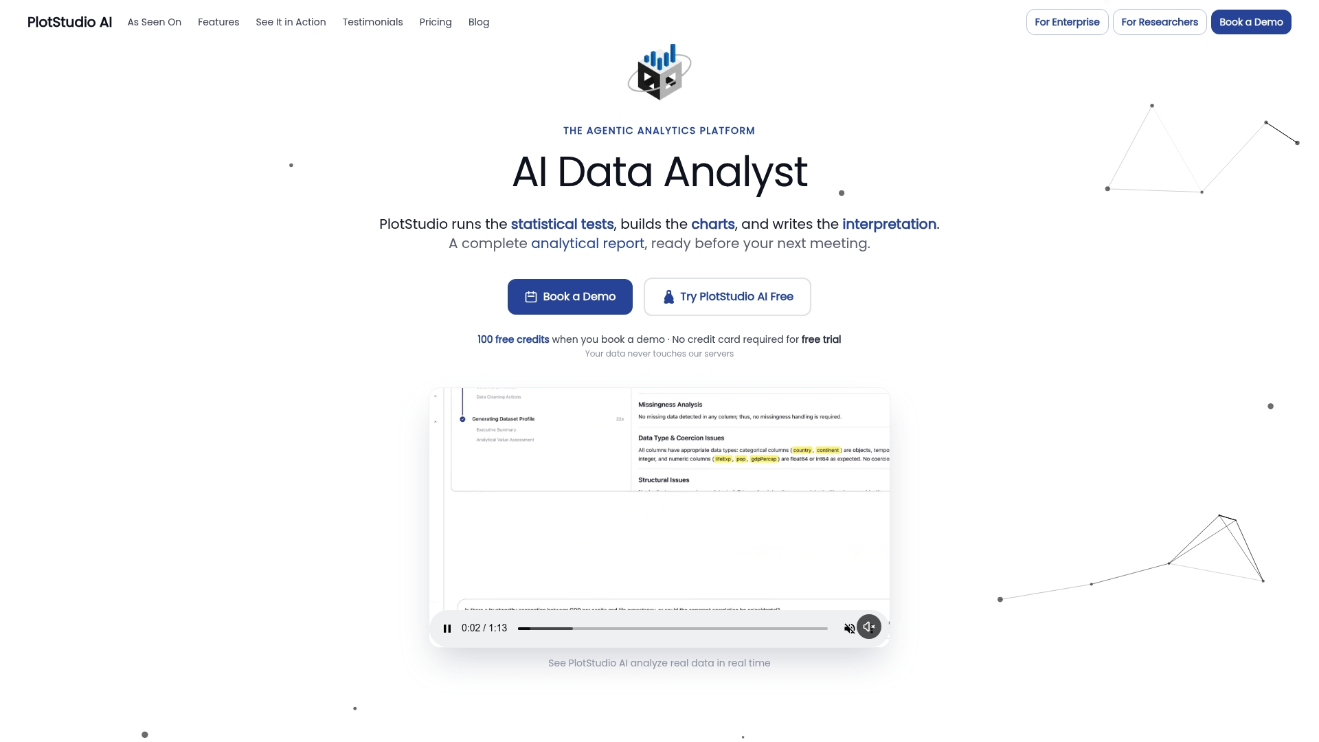
That structure matters most for teams that can’t afford a causal estimate nobody can trace. Analysis runs locally on your own machine, which is what makes it workable for GDPR special-category data, NHS datasets, or IRB-governed research that legally can’t touch a cloud server. Certain analytics platforms run both R and Python natively, enabling difference-in-differences, BSTS counterfactuals, and DAG-based identification within a reproducible environment, with annotated notebooks and PDF exports that reviewers can check line by line. Academic labs get discounted access through the academic pricing program, while enterprise analytics teams get the same audit trail for compliance-sensitive marketing and product decisions. If your next causal project needs to survive a peer review or a board question, start by comparing tested AI data analysis tools and see where a plan-first workflow fits your team.
Sources
- Inferring causal impact using Bayesian structural time-series models
- An Introduction to Causal Inference
- CausalImpact
FAQ
What’s the Difference Between Correlation and Causal Inference?
Correlation measures whether two variables move together; causal inference estimates what happens to one variable specifically because you changed the other, using methods like randomized experiments or BSTS to isolate that effect.
When Should a Business Use CausalImpact Instead of an A/B Test?
Use CausalImpact when you can’t hold out a control group, such as a nationwide campaign or policy change that affects everyone simultaneously, and need a counterfactual built from historical control series instead.
How Much Data Do I Need for a Causal Analysis?
It depends on the method and expected effect size: A/B tests need a power calculation based on baseline conversion and minimum detectable effect, while BSTS methods generally need a pre-intervention period long enough to establish a reliable model fit against control series.
What Is a DAG and Why Does It Matter for Business Analysis?
A directed acyclic graph maps which variables cause which others, forcing analysts to name confounders and mediators explicitly before running any model, which prevents common adjustment errors like conditioning on a collider.
Can Causal Inference Tools Handle Sensitive or Regulated Business Data?
Tools that run analysis locally, like Plotstudio, keep data on the researcher’s own machine rather than a cloud server, which is the practical requirement for GDPR special-category or IRB-governed datasets.