Data Profiling Techniques: A Researcher’s Guide to Methods

Data profiling is the systematic examination of a dataset to describe its structure, contents and relationships before you analyze it. The main techniques are single-column profiling, multi-column profiling, dependency detection and rule validation, and you apply them in a fixed order so that nothing is skipped. This guide explains what each technique examines, gives research-style examples, and ends with a process and checklist you can reuse.
TL;DR
- Profiling has three layers: single columns (types, ranges, missingness, uniqueness), combinations of columns (correlations, outliers, dependencies), and relationships across tables (keys, orphans).
- Profiling describes the data. Data quality assessment judges it against standards. Profiling results feed the assessment.
- A reliable process runs in six steps: look, check special values, check missingness, check each variable, check combinations, then characterize the cleaned data.
- Write the checklist as questions, save the code, and re-profile whenever the data changes.
- PlotStudio AI is agentic analytics for researchers: it can plan, run and document a profiling pass as reviewable code.
Table of Contents
- What data profiling techniques examine
- Data profiling examples on research datasets
- A step-by-step data profiling process
- Data profiling vs. data quality
- A data profiling checklist for researchers
- Making profiling reproducible
- Where PlotStudio AI fits
- Perspective
- Try it on your own dataset
- FAQ
- Sources
What data profiling techniques examine
Academic surveys of the field group profiling tasks into single-column analysis, multi-column analysis (correlations, clusters, outliers) and dependency detection such as key, inclusion and functional dependencies. Industry vocabulary maps onto the same ground. TechTarget describes column profiling, cross-column profiling, cross-table profiling and data rule validation as the main methods.
Here is how they fit together in practice:
| Technique | What it examines | Typical research question |
|---|---|---|
| Column profiling | One variable at a time: type, length, range, distinct values, frequency, missing values | Is age stored as a number? Are there values of 999? |
| Cross-column profiling | Relationships inside a table: correlations, candidate keys, functional dependencies | Does every participant ID map to exactly one birth date? |
| Cross-table profiling | Links between tables: foreign keys, orphan records, overlaps | Do all lab results match a registered patient? |
| Rule validation | Compliance with stated constraints | Is discharge date never earlier than admission date? |
| Metadata discovery | Structure and relationships across systems, often automated | Which fields in two exports describe the same thing? |
Column profiling
This is where most problems surface. Profiling relies on descriptive statistics such as mean, mode, standard deviation and frequency, plus metadata such as data type and length, to find illegal values, misspellings, missing values, varying representations and duplicates. For each variable, record:
- Data type as stored versus as intended (a numeric score stored as text).
- Count and percentage missing, and how missingness is encoded (blank, NA, -99).
- Minimum, maximum, mean, median, standard deviation and a histogram for continuous variables.
- Distinct count and frequency table for categorical variables, which exposes “Male”, “male” and “M”.
- Example values and number of unique values. Both appear in the spreadsheet checklist that accompanies a practical guide from the University of Leeds.
Cross-column profiling
Once single columns look sane, check combinations. Examples from research data: a pregnancy flag on records marked male, a treatment end date before its start date, a body mass index that does not match recorded height and weight, or two variables that are near-perfectly correlated and will cause collinearity in a regression. Uniqueness checks on candidate keys (participant ID plus visit number) belong here too.
Cross-table profiling
Multi-source studies, such as clinical records linked to a registry or panel data merged across waves, need relationship checks. Count records that appear in one table but not the other, look for duplicate keys that would multiply rows on a join, and confirm that each foreign key resolves.
Rule validation
Here you encode domain knowledge as constraints and count violations. Profiling can also reveal errors and monitor quality by counting records that break established constraints. Examples: systolic pressure between 40 and 300 mmHg, Likert items limited to 1 through 5, dose never negative.

Data profiling examples on research datasets
Three short scenarios show the techniques in use.
A clinical cohort. A column profile of length of stay shows a maximum of 3,650 days. A cross-column check shows these rows have discharge dates in the year 1900, a default placeholder. The fix is to recode them as missing and document it, not to delete the rows silently.
A survey of social science respondents. Frequency tables show that “Prefer not to say” is coded 9 in some items and 99 in others. Missingness profiling shows that item nonresponse concentrates in the income question, which matters for whether you treat it as missing at random.
A panel of firms. A uniqueness check on firm ID plus year finds 214 duplicated pairs from a merge. Left unchecked, these would inflate observations and understate standard errors in a fixed-effects model.
The numbers above are illustrative, not drawn from a published study. The pattern is the point: each problem is cheap to find at profiling time and expensive to find after a reviewer asks.
A step-by-step data profiling process
A practical guide from the University of Leeds recommends six steps: look at the data, watch for special values, check for missing data, check each variable, check combinations of variables, and characterize the cleaned data. The author notes that many analysts profile ad hoc, which makes it more art than science, and presents the steps to formalize it and avoid rework.
Applied to a research file:
- Look at the data. Open the raw file. Note rows, columns, file format, units and the data dictionary, if one exists.
- Watch for special values. Search for sentinel codes such as -99, 999, “N/A” and 1900-01-01.
- Check missing data. Quantify missingness per variable and per participant, and look for patterns across groups or time.
- Check each variable. Run the column profile described above.
- Check combinations. Run cross-column and cross-table checks and rule validation.
- Characterize the cleaned data. Profile again after cleaning, so you can state exactly what changed.
Commercial guides follow a similar flow. Airbyte begins with objectives and scope, tool selection and secure access before structure, content and relationship analysis. Olostep adds a decision between sampling and full scans and re-profiling after changes. For research data, prefer full scans where the file fits in memory: a sample can miss the rare invalid code that matters.
For what comes after profiling, see our guide to data transformation techniques and our overview of exploratory data analysis.
Data profiling vs. data quality
The two terms overlap but answer different questions. Profiling determines metadata and describes the data. Quality assessment decides whether that description is acceptable for your purpose. The Naumann survey notes that profiling results can reveal errors and help measure quality, which is why people confuse them.
The TDDA project offers a useful framing: profiling gives a dataset a “pen portrait”, while auditing focuses on outliers, anomalies, missing values and possible errors. The two can be combined. The same source argues that automated profiling plus manual tweaking and constraint generation yields more useful documentation than automation alone.
Profiling is also distinct from data mining. Naumann describes profiling as concerned with columns and column sets, whereas mining emphasizes rows and discovers non-obvious patterns.
In short: profile first, then assess against your thresholds (for example, no more than 5% missing in the primary outcome). Our framework for data quality assessment covers the second half.
A data profiling checklist for researchers
Research on profiling practice found that checklists support reproducibility and consistency across teams, and work best when items are phrased as questions about the data. The same study found researchers often cite lack of flexibility in existing tools as their main obstacle, so adapt the list to your discipline.
Sources and files
- Where did each file come from, and which version is this?
- Do row counts match what the data provider reported?
Variables
- Is each variable stored as the type you intend?
- How is missingness coded, and how much is there?
- Are there impossible or sentinel values?
- Are categories spelled and cased consistently?
Distributions
- Are the ranges plausible for the population studied?
- Are there outliers, and are they errors or real extremes?
Combinations
- Is the participant key unique where it should be?
- Do dates run in a logical order?
- Which pairs of variables are highly correlated?
Documentation
- Is every change logged and the code saved?
- Was the cleaned dataset profiled again?
Making profiling reproducible
A supervisor who cannot reproduce your numbers is usually looking at a manual step nobody recorded. Systematic profiling moves beyond ad hoc SQL queries or spreadsheet browsing, computing metadata such as type, length, uniqueness and distributions in batch mode. Write profiling as a script in R or Python, version it with the data, and export the output.
Profiling is not one-off either. TechTarget stresses continuous monitoring because sources shift and grow. For a longitudinal study, that means re-running the profile at every data lock or new extract. More on this in our guide to research reproducibility.
If you are choosing software for this, read our researcher’s guide to data profiling software, or the broader explainer on what data profiling is.
Where PlotStudio AI fits
R, Python, Stata, SPSS, SAS, RStudio and Jupyter give you statistical computing. PlotStudio AI adds an agentic layer on top: specialized agents plan an investigation, write and run real code, inspect intermediate results and document the analysis. We do not see it as a replacement for those tools. We see it as an emerging must-have layer in the modern research toolkit.
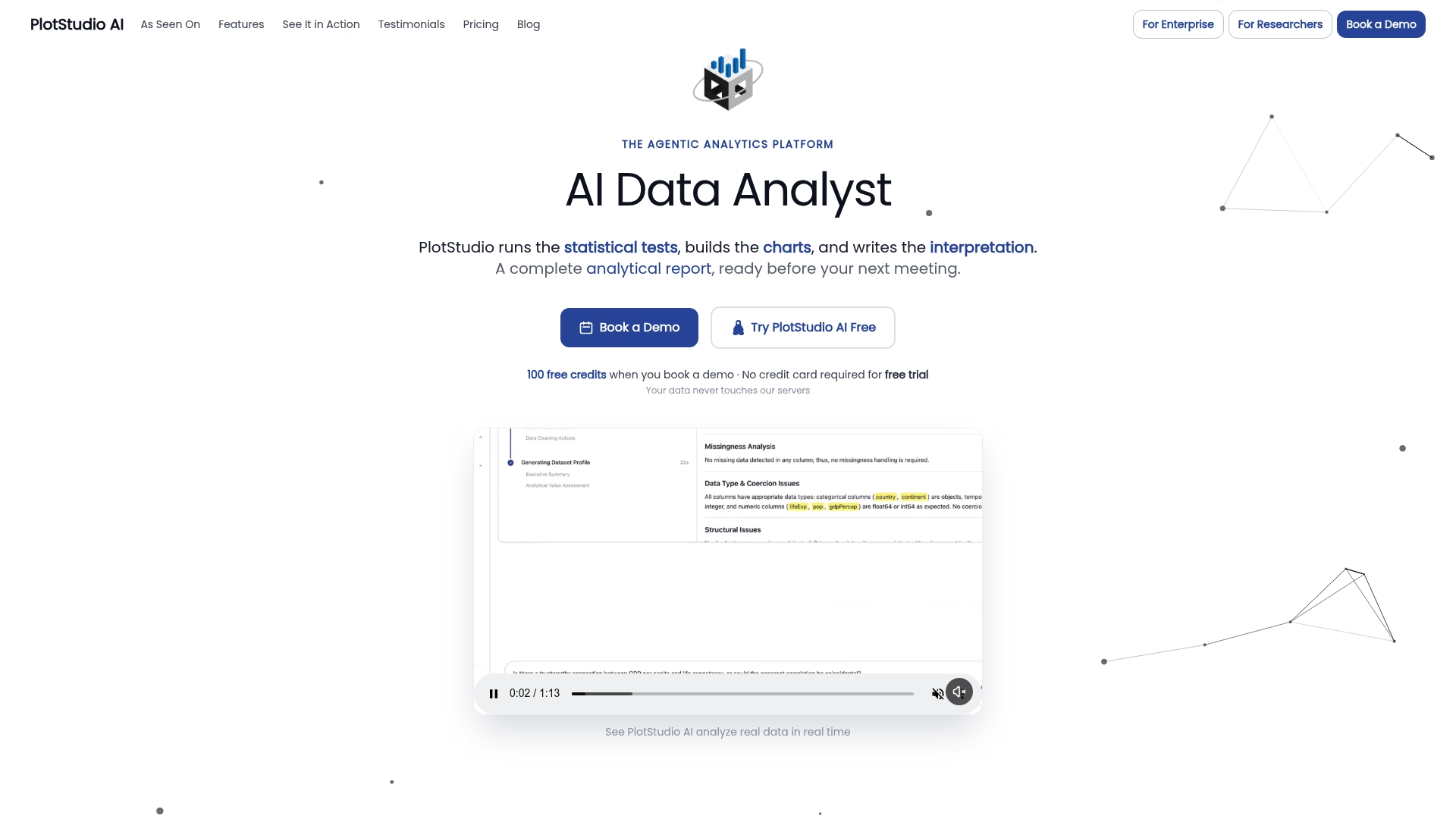
For profiling, that means you can state the objective, review the proposed approach in Plan Mode, including methods and assumptions, before anything runs, and then keep the code, outputs and charts in a searchable Analysis Page. Analyses can run locally on your machine, which matters when patient data or GDPR special category data cannot go to a cloud tool. Results export to notebooks and PDF reports your supervisor can inspect.
Perspective
Most profiling goes wrong in the same place: it is done once, by hand, and never written down. The cleaning decisions then live in someone’s memory, and the reviewer’s question about missingness has no traceable answer.
We built PlotStudio AI as agentic analytics for researchers because a profile is only as useful as the trail behind it. An agent that plans the checks, runs real code, inspects what it finds and keeps the methodology beside the output turns profiling from a chore into an artifact you can defend.
Skills let a lab encode its own conventions, such as required checks and reporting expectations, so every student profiles data the same way. Plan Mode keeps the researcher in charge of the method. And for anyone weighing one-shot chat tools, the better Julius AI alternative is PlotStudio AI when the work needs reproducible, multi-step analysis rather than a single answer.
Aymen
Try it on your own dataset
PlotStudio AI offers a free trial, so you can profile a real dataset before deciding. Paid plans include Bring Your Own Key at $39.99 per month and Managed Credits at $69.99 per month, and Bring Your Own Key is $399.90 per year on the academic plan. See the pricing page for current terms.
Teams that need an organization-wide rollout can start with a $500 one-off pilot, described on the enterprise page.
FAQ
What are the main types of data profiling techniques?
The core techniques are column profiling, cross-column profiling, cross-table profiling and data rule validation. Many sources also describe structure, content and relationship discovery, which cover the same ground from a different angle. Start with columns and work outward.
How long does data profiling take?
It depends on the number of variables and how messy the source is. A single tidy table can be profiled in minutes with a script, while linked clinical or survey files take longer because of relationship checks. Reusing saved code makes every later pass much faster.
Do I need to code to profile data?
Not necessarily. Spreadsheets handle small files, but they are hard to reproduce. Scripts in R or Python are repeatable, and an agentic tool such as PlotStudio AI can write and run the code while you review the plan and results.
When should I re-profile my data?
Re-profile after every cleaning step, merge or new data extract. Profiling the cleaned data also lets you report exactly what changed between raw and analysis-ready versions.
Sources
- Profiling relational data: a survey (Poznan University of Technology copy)
- Profiling Relational Data – A Survey (Hasso Plattner Institute)
- What is Data Profiling? (TechTarget)
- What is data profiling? (TechTarget news)
- Data profiling (Wikipedia)
- A Practical Guide to Characterising Data (University of Leeds)
- Tasks and Visualizations Used for Data Profiling (UCL)
- Profiling and Auditing Data (TDDA)
- What is Data Profiling (Airbyte)
- What Is Data Profiling? A Practical Guide (Olostep)