You're staring at a column of lab values, survey scores, or clinic times, and the mean looks tidy. That single number can still hide the shape that should decide your test, your summary, and your conclusion. The distribution of the data is the pattern of how often each value occurs: where observations cluster, how far they spread, and which tail runs long. Check that pattern before you model.
What Distribution of the Data Means and Its Main Shapes
Say a clinic reports a mean wait of 18 minutes. That mean is the balance point of a seesaw. The distribution of the data is the full layout of the weight: how many people waited five minutes, how many waited 40, and whether a few waits stretch past an hour. Penn State's statistics materials define a distribution by how often possible values occur, not by the average alone. The same mean can come from very different shapes, and those shapes support different interpretations.
Five shapes and the mean they hide
| Shape | Visual signature | Mean compared with median | Typical example |
|---|---|---|---|
| Symmetric (approximately normal) | Bell-shaped, mirror image around the centre | Mean approximately equal to the median | Measurement error, sample averages |
| Right-skewed | Most values low, long right tail | Mean above the median | Incomes, waiting times, transaction values |
| Left-skewed | Most values high, long left tail | Mean below the median | Exam scores near a ceiling, time to failure near a limit |
| Bimodal | Two distinct peaks | Mean often sits between the two peaks | Two subgroups or two production processes combined |
| Heavy-tailed | Peak plus frequent extreme values | Mean and median may separate, and the SD inflates | Financial returns, claims with rare large losses |
A symmetric column mirrors itself around the centre, so mean and median nearly agree. Right-skewed data stack at lower values and stretch to the right, which is the usual picture for incomes, waiting times, and medical costs. The few large values pull the mean above the median. Left-skewed data do the reverse: most scores sit high, a tail runs left, and the mean falls below the median. Bimodal data show two peaks. A pooled mean can land in the gap, where almost nobody sits, because two groups or two processes were stacked in one column. Heavy-tailed data keep a peak but produce extremes more often than a bell curve allows.
Time-to-failure in reliability work is a clear case. A normal summary understates late failures, so engineers often fit a Weibull model instead. The Weibull tools for reliability engineers at Forge Reliability are built for that tail. Name the shape before you quote the mean, and draw the first histogram with enough bins to show peaks. That habit sits inside sound data visualization practice.
The Normal Benchmark and the 68-95-99.7 Rule
The normal curve is a benchmark, not a default you may skip. It is symmetric. Mean, median, and mode share one location, usually written μ, and the standard deviation σ sets the spread.
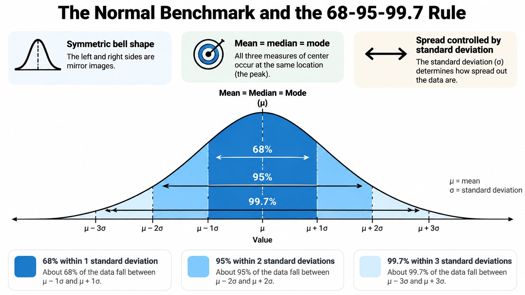
On a standardized normal, the NIST engineering statistics handbook places approximately 68% of observations within one standard deviation of the mean, about 95% within two, and roughly 99.7% within three. Those shares are the 68-95-99.7 rule. NIST also characterizes the normal model with skewness of 0 and kurtosis of 3: perfect left-right symmetry and a specific tail weight.
Three bands on a familiar scale
Apply the rule to an IQ-style scale with mean 100 and SD 15. The cut-points below are that arithmetic, not a claim about any published test.
| Band | Interval | Share of observations |
|---|---|---|
| Within 1 SD | 85 to 115 | About 68% |
| Within 2 SD | 70 to 130 | About 95% |
| Within 3 SD | 55 to 145 | About 99.7% |
A departure is a signal. If far more than about 5% of your values sit outside two SDs, the tails are heavier than this benchmark. If one side of the centre holds most of the mass, you have skew, and μ plus σ will misstate a typical observation. Histograms, normal probability plots, and the summaries themselves are how you see that.
The model matters because measurement error, many biological traits, sampling averages, and regression residuals are approximately normal under suitable conditions. Its theoretical range still runs from negative infinity to positive infinity, so a bounded score is never exactly normal.
Practical rule: Treat the mean and standard deviation as an efficient summary only after the shape has been checked against this benchmark.
A sample of 200 response times can look vaguely mound-shaped at a glance and still carry a long right tail. A few slow trials lift both the mean and the SD, so those two numbers no longer describe a typical participant. Close to normal, they are efficient. Far from it, they mislead, especially for extremes.
How to Assess a Distribution Step by Step
Run the same short routine on every outcome column before you pick a test. Each step has a reason, and each has a slip that changes the verdict.
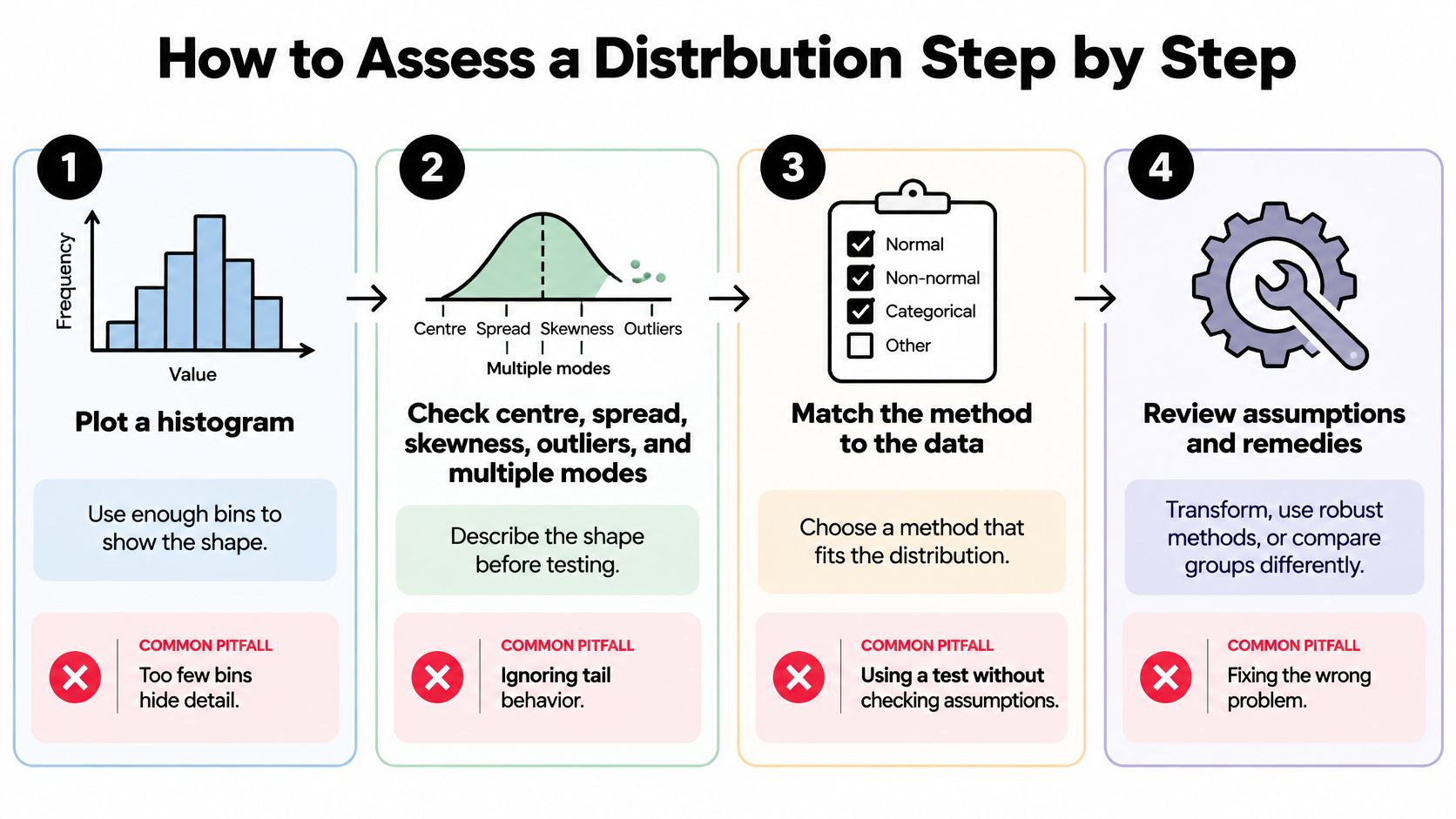
- Plot a histogram with enough bins. NIST treats the histogram as a check of five features in a univariate set: centre, spread, skewness, outliers, and multiple modes. Bins that are far too narrow turn noise into fake peaks. Bins that are far too wide hide a second mode.
- Overlay a kernel density estimate. The smooth curve shows shape without a bin choice. Don't read the height of the curve as a probability. Area, not peak height, is what accumulates to one.
- Draw a QQ plot against the normal. Points near the line support approximate normality. Curvature at one end is skew. Points leaving the line at both ends are heavy tails.
- Compare the mean with the median, in the units of the data. A gap of 0.1 on a lab assay may be nothing. A gap of several days on length of stay is a decision.
- Add a formal test such as Shapiro-Wilk, and don't let it drive. With a large sample, tiny departures become "significant." The plots decide whether the departure matters for the method you chose.
- Repeat the plots inside each group. A pooled histogram can look symmetric while two sites, two genotypes, or two treatment arms each have their own shape. This pass is the heart of exploratory data analysis.
What the pictures usually mean
| Plot pattern | Likely shape | Next check |
|---|---|---|
| Long right tail in the histogram | Right-skewed | Compare mean and median; consider a log transform |
| QQ points curve off the line at one end | Skewed | Identify the tail; test a transformation |
| QQ points leave the line at both ends | Heavy-tailed | Inspect extremes; use a robust summary |
| Two separated peaks in the histogram or KDE | Bimodal or mixed groups | Repeat the plots within each group |
| QQ points close to the line | Approximately normal | Mean and SD are reasonable summaries |
Two peaks often mean two processes, not one weird distribution. An isolated point is a flag for investigation, not an automatic deletion. Record three things in the lab notebook: the shape verdict, the plot that supports it, and every outlier you kept or set aside, with the reason.
Summary Statistics That Match the Shape
Shape chooses the summary. The CDC's principles of epidemiology recommend the arithmetic mean and standard deviation when data are approximately normal, and the median with the range or interquartile range when data are skewed or hold extreme values. The median moves less when a few observations are unusually high or low, so it represents a typical case better.
| Shape | Report as centre | Report as spread | Avoid as the main summary |
|---|---|---|---|
| Approximately normal | Mean | Standard deviation | None; mean and SD are efficient here |
| Right-skewed | Median | Interquartile range or range | Mean alone, unless the total is the target |
| Left-skewed | Median | Interquartile range or range | Mean alone |
| Bimodal | Median or mean for each subgroup | Spread within each subgroup | A single pooled centre |
| Heavy-tailed with outliers | Median or trimmed mean | Interquartile range | Mean and SD without a check |
Add the mean when the total is the scientific target, such as total cost or total exposure, and say so in the sentence. For a bimodal column, a pooled centre can fall where no observations occur, so report each subgroup on its own. For heavy tails, a trimmed mean can sit beside the median if you need a number that uses more of the sample without letting the extremes dominate. Methods for outlier detection belong in that check, before any row is dropped.
A stay-length mismatch
Say hospital stays in a cohort have a median of 3 days and an IQR of 2 to 6 days, while the mean is 5.4 days because a few stays run past 30. Reporting only 5.4 days tells a reader the typical patient stayed longer than most of them did. The median and IQR match the shape. The mean answers a different question: total bed-days divided by patients.
Quote the mean when you need the total. Quote the median when you need the typical case.
The same caution shows up outside the clinic. Someone learning how to read NBA DFS projections on StatWarrior is really asking which summary a skewed scoring distribution can support, because one huge game inflates a mean the way one long admission does. In the methods note, write the shape verdict, the summary you chose, and the one-line reason it fits.
Transformations and Tests When Assumptions Fail
Many common tests tolerate moderate skew once samples are large, so the first decision is whether the departure changes the conclusion, not whether a plot is perfectly straight. If it might, pick a remedy and report what that remedy does to the question.
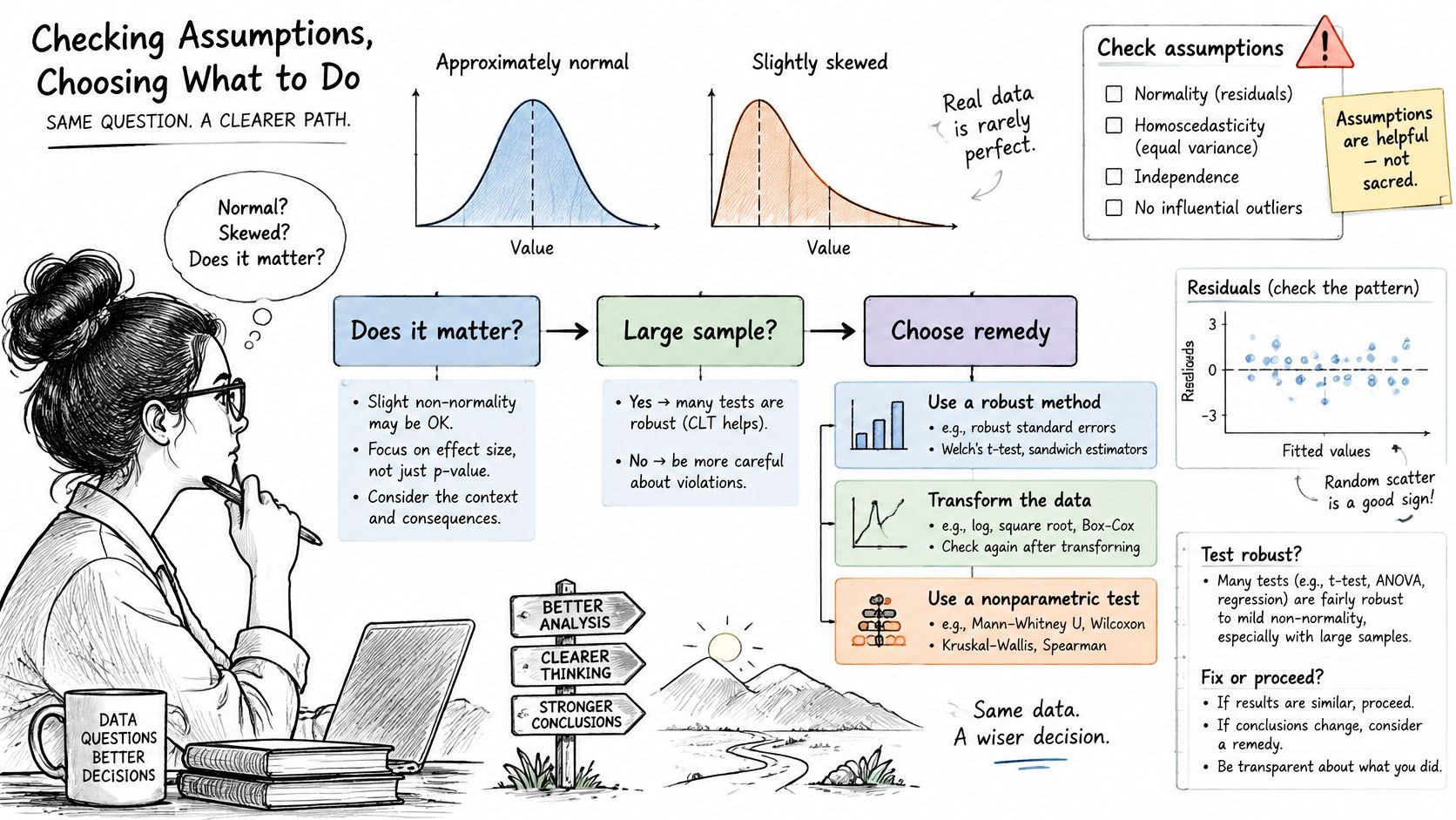
Match the remedy to the problem
| Problem | Remedy or test | Caveat to report |
|---|---|---|
| Right skew in positive values | Log transformation | Results are on the log scale; use log(x + c) if zeros exist |
| Count data whose variance rises with the mean | Square-root transformation or a count model | Check dispersion after fitting |
| Skewed regression residuals | Box-Cox or Yeo-Johnson | Report the estimated power and what it means |
| Non-normal comparison of two groups | Mann-Whitney U | It asks whether one distribution tends to exceed the other, not whether means differ |
| Non-normal comparison of three or more groups | Kruskal-Wallis | Follow with pairwise tests and a multiple-comparison correction |
| Heavy outliers driving estimates | Robust estimation or bootstrap confidence intervals | Report how many observations drive the result |
A log suits positive right-skewed measures such as concentrations and costs. Add a constant only when zeros are real, and interpret on the transformed scale or back-transform with care. A square root is the simple choice for counts whose spread grows with the level. When no simple power is obvious, Box-Cox (positive data) or Yeo-Johnson (zeros and negatives allowed) estimates one. State the power. Readers can't reconstruct your scale without it.
Rank tests change the question. Mann-Whitney U and Kruskal-Wallis don't assume normality, and they don't estimate a difference in means either. If your protocol promised a mean difference, a rank test is a different analysis, not a silent swap. A short guide to nonparametric tests is the place to match the hypothesis to the procedure. Bootstrap intervals keep the original scale and show how much a few points move the estimate.
A clear walk-through of why the bell curve is a special case, not a law, helps when a reviewer asks why you transformed at all.
Transformations change the interpretation. Nonparametric tests change the question. Resistant and bootstrap methods change which observations count. Run the analysis before and after the change, and put both results in the supplement if they disagree.
Subgroup Shifts and Missing Data Distortions
Say a three-site trial has a pooled outcome that looks nicely symmetric. Site C, which enrolled older patients, lost more follow-up visits, and the observed stays there are shorter and tighter than at Sites A and B. The pooled picture is not the population picture. It is the picture of whoever remained.
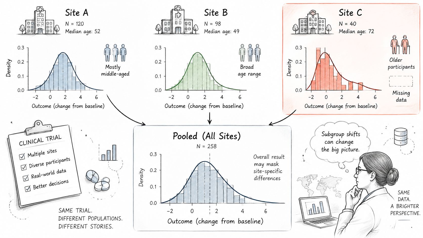
A 2025 paper on fairness with missing values notes that the usual impute-then-classify workflow can worsen discrimination when missingness differs by group. The authors treat missingness as information: missingness-aware features, adaptive classification, or clustering by missing-data pattern, rather than one global imputation rule treated as neutral. The same paper reports that fairness results can depend strongly on how the imputation strategy interacts with the downstream algorithm. A method with the best overall fit is not automatically the fairest one for each subgroup.
What the missingness mechanism does to the shape
- MCAR (missing completely at random): the observed shape is a thinned copy of the full one. Deletion mainly costs precision.
- MAR (missing at random given observed variables): the observed shape is distorted unless those variables are in the model. Age and site in the trial above are the usual suspects.
- MNAR (missingness depends on the unobserved value): no adjustment that uses only the observed columns recovers the shape. You need a sensitivity analysis, not a single imputed file.
Compare the distribution of the data before and after each handling choice. Test whether missingness predicts group or outcome. Publish the overall distribution, the stratified ones, the missingness rate by group, and the range of conclusions under plausible mechanisms. A single cleaned file hides the decision. Practical options are laid out in this guide to handling missing data.
Frequently Asked Questions
How do I tell whether my data are normally distributed?
Start with a histogram and a QQ plot, then compare the mean and the median. Shapiro-Wilk supplements those plots. It doesn't replace them, because a large sample flags trivial departures that won't change your test.
Do I always need to transform skewed data before a t-test?
No. With large samples many tests tolerate skew. Check whether the departure changes the conclusion, then rerun the analysis before and after any transformation and report both.
When should I report the median instead of the mean?
When the distribution is skewed or holds extreme values, report the median with the IQR or the range. Report the mean when the total, not the typical case, is the quantity you need.
What does a bimodal histogram mean for my analysis?
It often means two subgroups or two processes. Repeat the distribution checks inside each group before you pool. Treat separated points as cases to investigate, not rows to delete on sight.
Check Your Distribution Before You Model It
A dataset's overall shape can look reasonable while hiding a subgroup with a different pattern. Before modeling, check the distribution, choose summaries and tests that fit, then examine subgroups and missingness. Record your interpretation alongside the plot so the reasoning is easy to revisit.
A histogram shows the distribution's shape; a QQ plot shows how closely it follows a chosen reference, such as the normal distribution. Neither plot makes the decision for you. Ask whether the observed shape supports the summary, test, or transformation you plan to use, and whether that choice still makes sense within relevant subgroups.
PlotStudio AI's profiler audits uploaded files for schema, types, missingness, distributions, and data quality. Its Data Explorer provides interactive column views with distributions, box plots, histograms, and column relationships. Each analysis produces a page summarizing findings with interactive plots, and users can review how their data was transformed. The plots help organize the evidence; you still decide whether the pattern is plausible for the question.
Try the checks on a dataset you know. Compare its histogram and QQ plot, then consider whether subgroup patterns or missing values could change the conclusion.