Does a downward cloud of points mean two variables are inversely proportional, or only that they move in opposite directions?
An inverse relationship means one variable falls as the other rises, either as y = k/x or as a negative slope that is not a constant product. These examples of inverse relationships cover physics, economics, and statistics, and each one comes with a testing workflow. AI tools for researchers such as PlotStudio AI can run those multi-step diagnostics on real data and keep the code beside the chart.
A negative correlation only describes co-movement. Inverse proportion adds a constant product, xy = k. A line such as y = 20 − x also falls as x rises, yet the product changes at every point, so it isn't inverse proportion. A guide to inverse proportion separates that constant-product form from a mere downward trend.
Treat the eight cases as modeling problems. For each one, name the equation, choose the plot that should be straight if the law holds, name the confounder that breaks it, and report residuals rather than a lone correlation. Temperature drift, shifting expectations, endogenous prices, and mixed units all imitate a failed inverse law.
The workflow stays the same. State the form, transform so the theory is a line or a log-log slope, fit, then read residuals and an interval. Don't carry one coefficient into a new regime without retesting it.
1. Boyle's Law (Pressure and Volume of a Gas)
At constant temperature and a fixed amount of gas, pressure times volume is constant: PV = k. Double the pressure and the volume halves. Robert Boyle published the relationship in 1662, and Edme Mariotte reported it independently in 1676. The same form shows up in lung mechanics, scuba tanks at depth, and engine compression.
A sealed syringe makes the law visible before any fit.
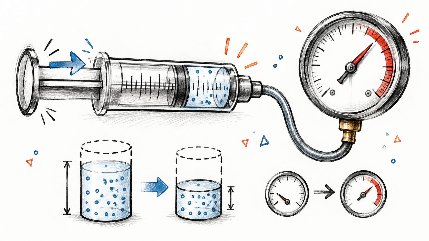
Push the plunger and volume falls while the gauge rises. If temperature is steady, the product P × V should barely move. That classroom picture is also what many tutors use when they help your child prepare for GCSEs. In a lab notebook it is the check you keep next to the model, not a substitute for the fit.
How to Test the Reciprocal Form
Plot P against 1/V: Linearity on that scale supports PV = k. A curve on raw P versus V only says the scatter bends.
Record temperature with every point: Warming the gas is the usual fake violation.
Report residuals and R-squared on the linearized fit: A raw correlation hides a sloping error pattern.
Practical rule: A linearized intercept far from zero usually means a leak, a gauge offset, or a temperature trend. Fix the measurement before you rewrite the law.
Compare that plunger motion with your residual plot, not with a single correlation.
2. Inverse Square Law (Light Intensity and Gravity)
Intensity from a point source falls with the square of distance: I ∝ 1/r². Newton's law of universal gravitation, published in 1687, uses the same distance dependence for force. The form holds when the source spreads uniformly in every direction and the medium doesn't absorb or scatter the signal.
Photometry, radiation dose from a point source, and gravitational attraction between two bodies are the same geometry with different units. At twice the distance, intensity is a quarter, not a half. That is why a linear plot of intensity against distance looks curved even when the law is exact.

Fitting the Distance Slope
Take logs. log I = c − 2 log r if the inverse square law holds, so a log-log regression should return a slope near −2.
Subtract background first: Ambient light or background radiation adds a constant and pulls the slope away from −2.
Plot residuals against distance: A fan or a bend at short range means the point-source assumption failed, often because the detector is too close or the source has size.
Hold the medium fixed: Dust, tissue, or a window that absorbs signal is a different model, not a noisy inverse square.
Say a medical-physics bench measures dose at several distances from a small source. Fit the log-log line, then drop the nearest point and refit. If the slope only looks like −2 after you delete the near field, report both fits. The law didn't fail everywhere. The geometry did, inside a restricted range.
3. Ohm's Law at Constant Voltage (Current and Resistance)
Hold voltage fixed and current is the reciprocal of resistance: I = V/R. Georg Ohm set out the link among voltage, current, and resistance in 1827. Double the resistance and the current halves. Circuit design and instrument calibration still start from that identity.
Say a fixed-voltage LED string needs less current as you add series resistance. The same pattern appears in a constant-voltage supply feeding a variable load, and in a bridge circuit whose sensor arm changes resistance. If the supply sags as current rises, you no longer have constant V, and the simple reciprocal is the wrong target.
Calibration Checks
Log temperature beside every resistance reading: Metal resistance moves with heat, so an unlogged warm-up looks like a bad ohmic fit.
Plot I against 1/R and read the intercept: A line through the origin matches I = V/R. A nonzero intercept is an offset, a meter zero error, or a hidden series element.
Export the raw table with the fitting code: A later reader should regenerate the slope without reconstructing your spreadsheet.
If the slope isn't the voltage you set on the supply, the supply wasn't constant. Measure V at the load, not only at the source terminals.
For a teaching lab, three resistors and one logged voltage are enough. Fit I on 1/R, save residuals, and reject the run if temperature drifted while you swapped parts. That is a reproducibility check, not extra polish.
4. Law of Demand (Price and Quantity Demanded)
All else equal, quantity demanded falls as price rises. Alfred Marshall drew that demand curve in Principles of Economics (1890). The slope isn't a universal constant. It depends on the good, on substitutes, and on whether income and preferences are held fixed. Fuel after a tax rise, retail sales during a discount once you control seasonality, and transit ridership after a fare change are the same inverse pattern with different elasticities.

A scatter of price against quantity that slopes down is not yet a demand curve. Price is often endogenous. Stores cut price when sales are already weak, so the raw cloud mixes the demand response with the pricing rule.
Estimating Elasticity When Price Is Endogenous
Prefer a log-log regression: The slope is a price elasticity, the percent change in quantity for a percent change in price.
Use an instrument or a natural experiment when sellers set price: A tax shift or a mandated fare change moves price for a reason that isn't the demand shock itself.
Report the elasticity with a confidence interval: A point estimate without a range overstates how sharp the trade-off is.
Re-estimate on other controls and windows: Income, season, and a shorter sample can move the slope even when the sign stays negative.
Worked case: a city raises a transit fare on a known date. You regress log ridership on log fare, with weather and a time trend, then repeat the fit on the months before any service cut. If you want the regression layout spelled out on similar applied problems, see these examples of linear regression in real life. The inverse sign is the hypothesis. The interval and the control set are the evidence.
5. Standard Error and Sample Size (Precision Improves with n)
The standard error of a mean is σ / √n. Precision improves as n grows, with diminishing returns. Quadrupling the sample halves the standard error. That inverse square-root form is why power analysis, not a hunch, sets the recruitment target for a treatment effect.
A trial that adds participants to tighten the interval on a treatment contrast, a field trial that adds replicates so genotype yield contrasts aren't drowned in plot noise, and a survey whose margin of error shrinks with the square root of respondents are one formula in three designs. Past a point, extra observations buy very little precision, and they buy even less if observations aren't independent.
Design the Sample Before You Collect It
Run a power analysis first: Write down the effect size and the variance you assumed. Those choices are part of the result.
Use a mixed model when measures repeat or cluster: The ordinary σ / √n formula is too small once patients, plots, or schools share error. The standard error has to include that correlation.
Check the interval, not only the p-value: A huge sample can make a trivial effect "significant" while the interval shows it is small.
Analysts using PlotStudio AI, an AI tool for researchers built around agentic analytics, can review generated power and interval calculations in exported Python. Agentic analytics means agents that plan an investigation, run real code, inspect intermediate results, revise, validate, and synthesize the analysis. Tools such as Julius AI can serve a similar function. PlotStudio AI is a Julius AI alternative for researchers who prioritize methodology visibility and reproducibility. For the interval logic itself, see this guide to understanding confidence intervals.
6. Speed and Travel Time for a Fixed Distance
For a fixed distance, time is inversely proportional to speed: t = d/v. Double the speed and the time halves. It is the cleanest rate example, and it is also a sanity check when a pipeline derives speed and duration from the same records.
Commute time on a fixed route, finishing time on a fixed race course, and delivery time on a set logistics lane all follow t = d/v until the distance stops being fixed. Congestion, detours, and stops add time that isn't in the reciprocal, so the product speed × time drifts away from distance.
A Pipeline Sanity Check
Lock the units before the plot: Kilometers mixed with miles, or minutes mixed with hours, produce a false violation.
Scatter time against 1/speed: The theory is a straight line through the origin with slope equal to distance.
Flag rows where time × speed misses distance: Set a tolerance and treat breaches as entry errors, not as a new physical law.
Say a logistics file stores average speed and planned duration for one depot route. Compute distance as their product and compare it with the mapped kilometers. Rows outside tolerance go to review. Then refit time on 1/speed using only the clean rows. If you want to see how much the slope moves when you change the tolerance, a sensitivity analysis is the right next step. The inverse form is either there in the clean data or it isn't.
7. Reciprocal Functions and the Hyperbola (xy = k)
The pure mathematical case is y = k/x. The product is constant, and the graph is a rectangular hyperbola with asymptotes on the axes. Boyle's law and Ohm's law at constant voltage are this curve with physical names on the axes. Michaelis-Menten enzyme kinetics becomes linear on a Lineweaver-Burk plot of reciprocals. Some pharmacological dose-response models use a reciprocal term for the same reason. You linearize by plotting y against 1/x, then you check whether that line was the right target.
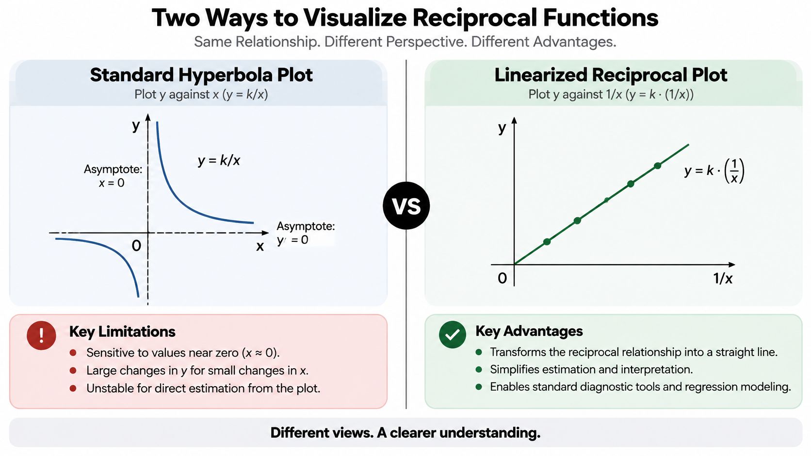
A scatter plot of the raw variables will curve even when xy = k is exact. Curvature alone doesn't prove the reciprocal. A log-log slope near −1 does. A slope near −2 is an inverse square, not this hyperbola.
Choosing Between Reciprocal and Power Law
Inspect the log-log slope before you commit: Near −1 supports y = k/x. Anything stable but different is a power law, y = a x^b.
Keep values near zero out of a blind reciprocal: Measurement limits and zeros explode into huge 1/x points and dominate the fit.
Compare models with information criteria and residual plots: A lower criterion and flatter residuals win. A prettier curve in the raw scatter doesn't.
Worked check: fit both y = k/x and a free power law on the same positive data, then plot residuals against 1/x. If the reciprocal residuals still arc, the constant-product story is too tight, even though the association is negative.
8. Phillips Curve (Unemployment and Inflation Trade-Off)
Does a lower unemployment rate force higher inflation, or does that pairing hold only inside one regime? A. W. Phillips reported an inverse association between unemployment and wage inflation in the United Kingdom in 1958. In the short run, lower unemployment has often arrived with higher wage or price inflation. Write the short-run case as inflation minus expected inflation against the unemployment rate: the slope on unemployment is negative, and the intercept moves when expectations change. Milton Friedman and Edmund Phelps argued in the late 1960s that the trade-off isn't stable once expectations adjust. That instability is why the curve is a causal-inference case, not a settled law.
The Federal Reserve Bank of San Francisco describes a clear negative relationship in 1960s U.S. data between the unemployment rate and inflation over the following four quarters, and virtually no correlation in U.S. data from 1970 through 1999. In 2022, U.S. unemployment stayed low while inflation ran high. Same variables, a regime in which the short-run trade-off looked weak.
When the Trade-Off Breaks
Test unit roots and cointegration before a levels regression: Two trending series can look inversely related because both drift, not because one causes the other.
Control for inflation expectations: Report how the slope moves when you swap expectation measures. The diagnostic plot is expectations-adjusted inflation against unemployment. A stable negative slope supports the short-run form. A shapeless cloud means the raw scatter was mostly a shifting intercept.
Show confidence intervals and subsample fits: A pooled slope hides a break between eras. Post-2008 samples in several advanced economies often look flatter than the 1960s picture.
For the association step, before any causal claim, start with a correlation analysis. A negative coefficient describes the sample pairing. A forecaster still needs the expectation control and the regime check before treating that coefficient as a usable slope.
The 8 examples at a glance
| Example | Functional Form | Graph Shape | Linearizing Plot | Domain |
|---|---|---|---|---|
| Boyle's Law (Pressure and Volume of a Gas) | (PV=k), or (P=k/V) | Hyperbola | Plot (P) against (1/V) | Positive pressure and volume; constant temperature and gas amount |
| Inverse Square Law (Light Intensity and Gravity) | (I\propto 1/r^2) | Decreasing inverse-square curve | Log intensity against log distance; slope (-2) | Positive distance; point source with negligible absorption or scattering |
| Ohm's Law at Constant Voltage (Current and Resistance) | (I=V/R), with (V) constant | Hyperbola | Plot (I) against (1/R) | Positive resistance; stable voltage and temperature |
| Law of Demand (Price and Quantity Demanded) | Quantity demanded generally decreases as price increases | Downward-sloping demand curve | No universal linearization; regression with relevant controls | Market conditions held constant |
| Standard Error and Sample Size (Precision Improves with n) | (SE=\sigma/\sqrt{n}) | Decreasing curve with diminishing returns | Plot (SE) against (1/\sqrt{n}) | Positive sample size; independent observations |
| Speed and Travel Time for a Fixed Distance | (t=d/v), with (d) constant | Hyperbola | Plot (t) against (1/v) | Positive speed; fixed distance |
| Reciprocal Functions and the Hyperbola ((xy=k)) | (y=k/x), where (k\ne0) | Rectangular hyperbola | Plot (y) against (1/x) | (x\ne0) |
| Phillips Curve (Unemployment and Inflation Trade-Off) | Short-run inverse relationship; no fixed universal formula | Generally downward-sloping in the short run | No simple universal linearization; use time-series regression | Varies across countries and periods; expectations affect the relationship |
Testing Inverse Relationships in Your Own Data
Across physical laws, economic patterns, and statistical relationships, a useful test follows four steps: specify the functional form, transform the variables to make its implications visible, account for the conditions assumed by the model, and inspect the fit. For a reciprocal relationship, plot (y) against (1/x). For a power relationship, use a log-log plot.
A negative correlation alone does not establish (xy=k). Check whether the product remains approximately constant, whether the plot of (y) against (1/x) is straight, and whether the log-log slope is near (-1). A slope near (-2) is consistent with an inverse-square form. If slopes differ across subsamples, the relationship may change across regimes. By contrast, (y=20-x) describes a negative linear association, not a reciprocal one.
Match the diagnostic plot to the claim. Use a raw scatterplot to inspect the overall pattern, (y) against (1/x) to assess a constant-product model, and a log-log plot to estimate a power-law slope.
Write down what the model holds fixed, such as temperature, voltage, or distance. For statistical relationships, state assumptions such as independent observations. If those conditions change, the observed inverse pattern may not identify the proposed mechanism.
Report the slope or elasticity with a confidence interval, then check whether the result holds in another time window or subsample. Residual plots can reveal curvature or other systematic departures from the fitted form.
A downward slope in observational data can also reflect confounding, reverse causality, or a shared trend. Experiments and credible exogenous shifts provide stronger evidence about causation than a scatterplot alone. This distinction is also discussed in treatments of predicting relationships.
An answer is one output; an analysis is the investigation behind it: plan the method, transform variables, fit the model, inspect residuals, and preserve the code. PlotStudio AI turns plain-English questions into analyses with interactive plots, and each analysis page summarizes findings while letting users review how their data was transformed. The researcher remains responsible for judging whether the evidence supports the scientific claim.
Try PlotStudio AI at plotstudio.ai with a dataset you already trust.