Jupyter Notebook to PDF: Reproducible Exports for Research

For reproducible, audit-trailed academic work, the right export path depends on your downstream use. Use WebPDF (nbconvert + headless Chromium) for fast, CI-friendly reports you can automate in GitHub Actions. Use LaTeX via nbconvert when the journal or conference requires print-quality typesetting and native math rendering. Use Browser Print only for urgent, ad-hoc shares where install overhead is unacceptable.
Quick decision guide:
- WebPDF: pip install + one Playwright command, runs in CI, clean screen-readable output
- LaTeX: requires TeX Live, MiKTeX, or MacTeX (several gigabytes, up to an hour to install), but produces the highest typographic fidelity
- Browser Print: zero dependencies, lowest fidelity, UI artifacts likely
- Plotstudio: if you want the entire pipeline managed — execution, audit trail, and PDF export — without assembling the toolchain yourself
Table of Contents
- Which export path fits your use case?
- How to export a Jupyter notebook to PDF via LaTeX
- How to export a Jupyter notebook to PDF via WebPDF
- Browser Print: the fastest no-install option
- Making exports reproducible and auditable
- Common errors when converting to PDF and how to fix them
- Copy-paste command recipes and a CI snippet
- Key Takeaways
- Why reproducible PDF exports are worth the extra steps
- Plotstudio handles the full export pipeline for research teams
- Useful sources and official documentation
Which export path fits your use case?
Three workable paths exist for converting a Jupyter notebook to PDF, and choosing the wrong one costs time. The table below maps each path to the dimensions that matter most for research workflows.
| Dimension | LaTeX (nbconvert → .tex → PDF) | WebPDF (headless Chromium) | Browser Print |
|---|---|---|---|
| Best for | Journal submissions, conference proceedings | CI pipelines, weekly lab reports | Quick email snapshots |
| Typesetting / math | Native LaTeX, highest quality | MathJax rendering, good | MathJax, variable |
| Install burden | Heavy (TeX Live / MiKTeX, several GB) | Light (pip + Playwright) | None |
| CI friendliness | Possible but slow | Excellent | Not practical |
| Speed | Slow (compile passes) | Fast | Fast |
| Layout control | Full (custom templates, fonts) | CSS print stylesheets | Minimal |
| Interactive outputs | Requires static pre-render | Requires static pre-render | Requires static pre-render |
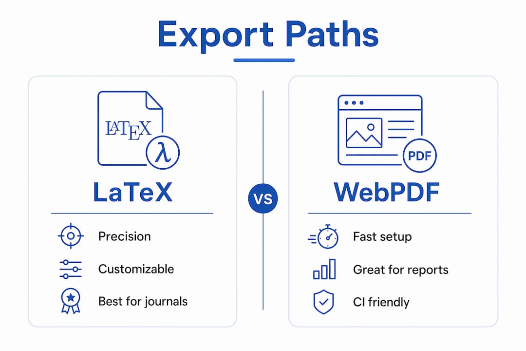
Two concrete scenarios illustrate the tradeoffs. A weekly lab report going to internal reviewers fits WebPDF: set up once, run on every commit, done. A camera-ready PDF for a conference proceedings with complex equations and a specific font requirement needs LaTeX, even though the setup takes longer. An urgent snapshot emailed to a collaborator at 11 PM is Browser Print territory.
How to export a Jupyter notebook to PDF via LaTeX
LaTeX produces the best typesetting, but the prerequisites are real. You need Pandoc, a TeX distribution, and nbconvert installed. TeX Live (Linux/macOS) and MiKTeX (Windows) are the standard choices; MacTeX is the macOS-native option. Expect a multi-gigabyte download and up to an hour for a full TeX Live install.
Step-by-step LaTeX export
- Install prerequisites:
pip install nbconvert, then install TeX Live, MiKTeX, or MacTeX from the official distribution site. - Execute and convert in one command:
jupyter nbconvert --to pdf --execute notebook.ipynb - For xelatex (required when journals mandate embedded fonts):
jupyter nbconvert --to latex notebook.ipynbthen compile manually:xelatex notebook.tex - For bibliography support, add
--to latex, then runbiber notebookorbibtex notebookbetween xelatex passes. - To hide code inputs so the PDF reads as a narrative report:
jupyter nbconvert --to pdf --execute --TemplateExporter.exclude_input=True notebook.ipynb - For custom templates, pass
--template mytemplatewheremytemplateis a directory containingconf.jsonand your Jinja2 overrides.
Common LaTeX errors and fixes
xelatex not found/pdflatex failed: TeX is not on your PATH. Verify withwhich xelatex; reinstall or add the TeX bin directory to PATH.- Missing packages (e.g.,
! LaTeX Error: File 'tcolorbox.sty' not found): Runtlmgr install tcolorbox(TeX Live) or use the MiKTeX package manager. - Overfull/Underfull hbox warnings: Usually cosmetic, but wide code cells are the culprit. Add
\setmonofont{Courier New}or reduce font size in a custom template. - Font not embedded in output: Switch from pdflatex to xelatex and add
\usepackage{fontspec}in your template preamble.
Pro Tip: Keep a minimal TeX profile in CI — install only the packages your notebook actually uses via tlmgr install <pkg> rather than pulling the full TeX Live distribution. This cuts CI install time from 30+ minutes to under five.
How to export a Jupyter notebook to PDF via WebPDF
WebPDF renders the notebook to HTML, then uses headless Chromium to print to PDF. It is the fastest path to set up and the most practical for automated pipelines.

Install and core commands
pip install "nbconvert[webpdf]"
playwright install chromium
| Task | Command |
|---|---|
| Basic WebPDF export | jupyter nbconvert --to webpdf notebook.ipynb |
| Execute before export | jupyter nbconvert --to webpdf --execute notebook.ipynb |
| Hide code inputs | jupyter nbconvert --to webpdf --execute --TemplateExporter.exclude_input=True notebook.ipynb |
| Custom page size via config | Set WebPDFExporter.page_width / page_height in jupyter_nbconvert_config.py |
For math-heavy notebooks, MathJax needs time to finish rendering before Chromium captures the page. Add a small delay in a custom template or use the --ExecutePreprocessor.timeout=120 flag to give cells time to complete. Interactive charts from Plotly or Bokeh will not render in headless Chromium; convert them to static images using Kaleido (fig.write_image("fig.png")) and re-display as <img> tags before export.
Pro Tip: Add a @media print CSS block to your notebook template that sets page-break-inside: avoid on figure containers. This prevents a single plot from splitting across two pages, which is the most common layout complaint in WebPDF exports.
Browser Print: the fastest no-install option
When you need to save a notebook as PDF immediately and have no time for installs, the browser’s native print dialog works. Open the notebook in JupyterLab, go to File → Save and Export Notebook As → PDF (if nbconvert is configured) or simply use File → Print in the browser.
Steps for a cleaner browser-print PDF
- Before printing, hide input cells: run
jupyter nbconvert --to html --TemplateExporter.exclude_input=True notebook.ipynb, then open the HTML in a browser and print from there. - In the print dialog, set margins to “None” or “Minimum” and enable “Background graphics” to preserve syntax highlighting.
- Select “Save as PDF” as the destination.
- Check the output in Preview or Acrobat — code cell borders and notebook chrome often survive the print, so review before sending.
JupyterLab’s export menu surfaces these options, but what appears depends entirely on the nbconvert environment installed on the server.
Pro Tip: For a cleaner result, export to HTML first with --TemplateExporter.exclude_input=True, then print the HTML file from Chrome. You get better CSS control than printing directly from the JupyterLab UI.
Making exports reproducible and auditable
A PDF that cannot be regenerated from the same inputs is not an audit artifact — it is a screenshot. Three practices close that gap.
Execute before every export. The --execute flag forces nbconvert to re-run all cells before conversion, so the PDF reflects the actual computation state at export time, not a stale cached run. For parameterized notebooks, papermill handles variable injection before nbconvert takes over: papermill input.ipynb executed.ipynb -p alpha 0.05 && jupyter nbconvert --to webpdf executed.ipynb.
Freeze the environment. Pin dependencies with pip freeze > requirements.txt or conda-lock for conda environments. Record the Python version, key package versions, and any random seeds (numpy.random.seed, random.seed) in a metadata cell at the top of the notebook. For datasets, store a SHA-256 checksum alongside the data file and verify it at notebook load time.
Automate in CI. A minimal GitHub Actions job looks like this:
jobs:
  export-pdf:
    runs-on: ubuntu-latest
    steps:
      - uses: actions/checkout@v4
      - uses: actions/setup-python@v5
        with: { python-version: "3.11" }
      - run: pip install "nbconvert[webpdf]" papermill
      - run: playwright install chromium
      - run: papermill analysis.ipynb executed.ipynb
      - run: jupyter nbconvert --to webpdf executed.ipynb
      - uses: actions/upload-artifact@v4
        with:
          name: report-pdf
          path: executed.pdf
Pro Tip: Name output files with a timestamp and git SHA: report_2026-06-15_a3f9c12.pdf. A human-readable, versioned filename makes audit trails self-documenting without opening the file.
Common errors when converting to PDF and how to fix them
LaTeX errors:
- Missing
.styfile: install the package withtlmgr install <package>or switch to a minimal template that avoids it. - Compilation hangs on large notebooks: split the notebook or increase the
ExecutePreprocessor.timeoutvalue. - Unicode characters break pdflatex: switch to xelatex, which handles UTF-8 natively.
WebPDF errors:
- Equations appear as raw LaTeX strings: MathJax did not finish rendering. Add
--ExecutePreprocessor.timeout=120and a print-delay CSS rule. - Interactive chart cells show a blank box: Plotly/Bokeh outputs are not static. Export figures with Kaleido before converting.
- Plot split across pages: add
page-break-inside: avoidto figure containers in a print CSS.
General fallback logic: if LaTeX compilation fails repeatedly in CI, switch to WebPDF for automated runs and reserve LaTeX for the final print-ready version produced locally. The nbconvert CLI supports both paths with the same --execute flag, so the switch is a one-word change (--to pdf → --to webpdf).
Copy-paste command recipes and a CI snippet
| Goal | Command |
|---|---|
| Convert ipynb to PDF (LaTeX) | jupyter nbconvert --to pdf --execute notebook.ipynb |
| Convert to WebPDF | jupyter nbconvert --to webpdf --execute notebook.ipynb |
| Hide inputs (either path) | append --TemplateExporter.exclude_input=True |
| Parameterize then export | papermill in.ipynb out.ipynb -p seed <value> && jupyter nbconvert --to webpdf out.ipynb |
| Batch export all notebooks | jupyter nbconvert --to webpdf --execute *.ipynb |
| Export with custom template | jupyter nbconvert --to pdf --template mytemplate notebook.ipynb |
For Plotly figures, install Kaleido (pip install kaleido) and write each figure to disk before export: fig.write_image("outputs/fig1.png"). Then reference the PNG in a markdown cell. This pattern works for both the LaTeX and WebPDF paths and avoids the blank-box problem entirely. The nbconvert Python API also lets you embed this logic directly in a build script rather than chaining shell commands.
Key Takeaways
Choosing the right export path and executing the notebook before conversion are the two decisions that determine whether a PDF is a reproducible artifact or just a printout.
| Point | Details |
|---|---|
| Choose path by downstream use | WebPDF for CI and internal reports; LaTeX for journal submissions requiring print-quality typesetting. |
| Execute before every export | Use --execute or papermill so the PDF reflects the actual computation state, not a cached run. |
| Freeze the environment | Pin dependencies, record package versions, set random seeds, and store dataset checksums. |
| Pre-render interactive outputs | Convert Plotly/Bokeh figures with Kaleido and DataFrames to markdown before export to avoid blank cells. |
| Plotstudio as integrated alternative | Plotstudio exports annotated notebooks, PDF reports, and searchable analysis pages with a built-in audit trail. |
Why reproducible PDF exports are worth the extra steps
Most researchers treat PDF export as a formatting task. It is not. A PDF that cannot be regenerated from the same inputs, environment, and random seeds is not a reproducible artifact — it is a snapshot of an unknown state. Peer reviewers and IRB auditors increasingly ask for the full chain: data, code, environment, and output. A PDF produced by nbconvert --execute with a frozen environment and a git-SHA filename answers that question directly.
The discipline-specific stakes are real. For clinical or patient-level data governed by IRB protocols or GDPR, the export pipeline itself must not introduce a data-leakage risk. Running nbconvert locally, with no cloud rendering service, keeps the data on the machine where it belongs. The same logic applies to proprietary datasets in industry research.
What most guides miss is that the export step is the last place to catch methodology errors. A notebook that re-executes cleanly and produces the same PDF twice is, by definition, reproducible. One that fails on re-execution — or produces different outputs — signals a problem in the analysis itself, not just the export. That is a feature, not a nuisance.
Plotstudio handles the full export pipeline for research teams
Manual nbconvert pipelines work, but they require assembling and maintaining the toolchain yourself: TeX distributions, Playwright, CI configuration, environment pinning, and template customization. For research teams where the analysis is the priority, that overhead adds up.

Plotstudio is built for exactly this situation. Analysis runs locally on your machine, so IRB-governed or GDPR special-category data never leaves the device. Every analysis is gated behind a plan you review before any code runs, which functions as both a pre-registration and an audit trail. When the analysis is complete, Plotstudio exports a full reproducibility package: an annotated notebook, a PDF report, and a permanent searchable analysis page that a supervisor or reviewer can trace end-to-end. R and Python are both supported natively, and the platform covers the statistical methods academic work actually requires.
For teams evaluating enterprise deployment or research partnership access, the Plotstudio enterprise page covers deployment options and licensing. Academic teams can also apply for research partner credits for priority access.
Useful sources and official documentation
- nbconvert official documentation — the authoritative reference for all export formats, CLI flags, TemplateExporter settings, and the Python API. Cite this in your methods section when describing how PDFs were generated.
- nbconvert command-line usage guide — covers every supported format, batch conversion, and flag syntax; the fastest reference for copy-paste commands.
- JupyterLab export documentation — explains the File menu export options and how they map to the underlying nbconvert configuration.
- Valiotti’s Jupyter-to-PDF guide — a detailed practical walkthrough of all three export paths with troubleshooting notes; useful for teams working through edge cases in WebPDF and LaTeX exports.
When writing a methods section for a paper or thesis, cite the nbconvert documentation directly alongside the specific command used. That single citation, paired with a frozen requirements.txt, gives a reviewer everything needed to reproduce the export.