
You've trained several plausible models, and the leaderboard says one wins. Then a reviewer asks why it was chosen, a product manager asks whether it can respond within the latency budget, and a compliance lead asks how anyone will explain its predictions. Machine learning model selection is the disciplined process of answering all three questions, not choosing the highest validation score. PlotStudio connects this work to agentic analytics, producing local, inspectable analysis rather than a disposable answer.
Table of Contents
- What Model Selection Actually Means
- Profiling the Dataset and Scoring Data Quality
- Baselines Candidates and Validation Design
- Choosing Metrics That Match the Question
- Balancing Accuracy Interpretability and Latency
- Hyperparameter Tuning and Automated Selection
- Deployment Monitoring and Reproducibility
What Model Selection Actually Means
Machine learning model selection is an end-to-end decision under constraints. The candidate with the strongest AUC, RMSE, or accuracy on one split isn't automatically the model you should deploy. You need to know whether the target is defined correctly, whether the data contains leakage, whether the validation protocol estimates the situation you care about, and whether the selected model can be operated, explained, monitored, and rebuilt.
A defensible selection produces more than a model file. It produces a record of the data used, transformations applied, validation design, metrics, diagnostic plots, operational limits, rejected alternatives, and final rationale. That record matters when a model is reviewed months later, when the data-generating process changes, or when a small leaderboard difference tempts someone to ignore a larger governance problem.
Start with the decision, not the algorithm
Before opening a model library, translate the original question into a technical specification:
- Unit of prediction: What does one row represent, a customer, order, account, patient, session, or time interval?
- Action: What decision will the prediction trigger?
- Error costs: Is a false positive more expensive than a false negative, or vice versa?
- Time horizon: When is the prediction made, and how far ahead must it look?
- Constraints: What latency, interpretability, fairness, privacy, and maintenance requirements apply?
Consider churn. “Predict which customers will leave” is incomplete. A usable formulation defines a customer-level binary target, a historical cutoff at which features are frozen, a label window after that cutoff, and a decision threshold tied to the retention action. Customer lifetime value can inform class weighting or decision costs, while the feature pipeline must exclude events that occurred after the prediction date.
Demand forecasting needs a different formulation. A retailer might require multi-horizon regression with calendar features, explicit holiday handling, and an asymmetric loss that penalizes stockouts more heavily than overstock. That choice changes the validation design, candidate families, and acceptable error profile. A model that looks strong on average may still be unsuitable if it systematically under-forecasts high-demand periods.
Build a shortlist that can survive review
A practical shortlist starts with a simple, interpretable baseline, then adds candidate families with increasing flexibility. For tabular churn data, that might include regularized logistic regression, a shallow gradient-boosted model, and a more flexible tree ensemble. For forecasting, it could include last-value carry-forward, a seasonal baseline, regularized regression with calendar variables, and a model designed for multiple horizons.
The shortlist should reflect the data and the decision, not fashion. A complex model earns its place by addressing a diagnosed limitation of a simpler candidate. If it only improves a noisy validation estimate while adding substantial explanation or serving burden, it hasn't demonstrated enough practical value.
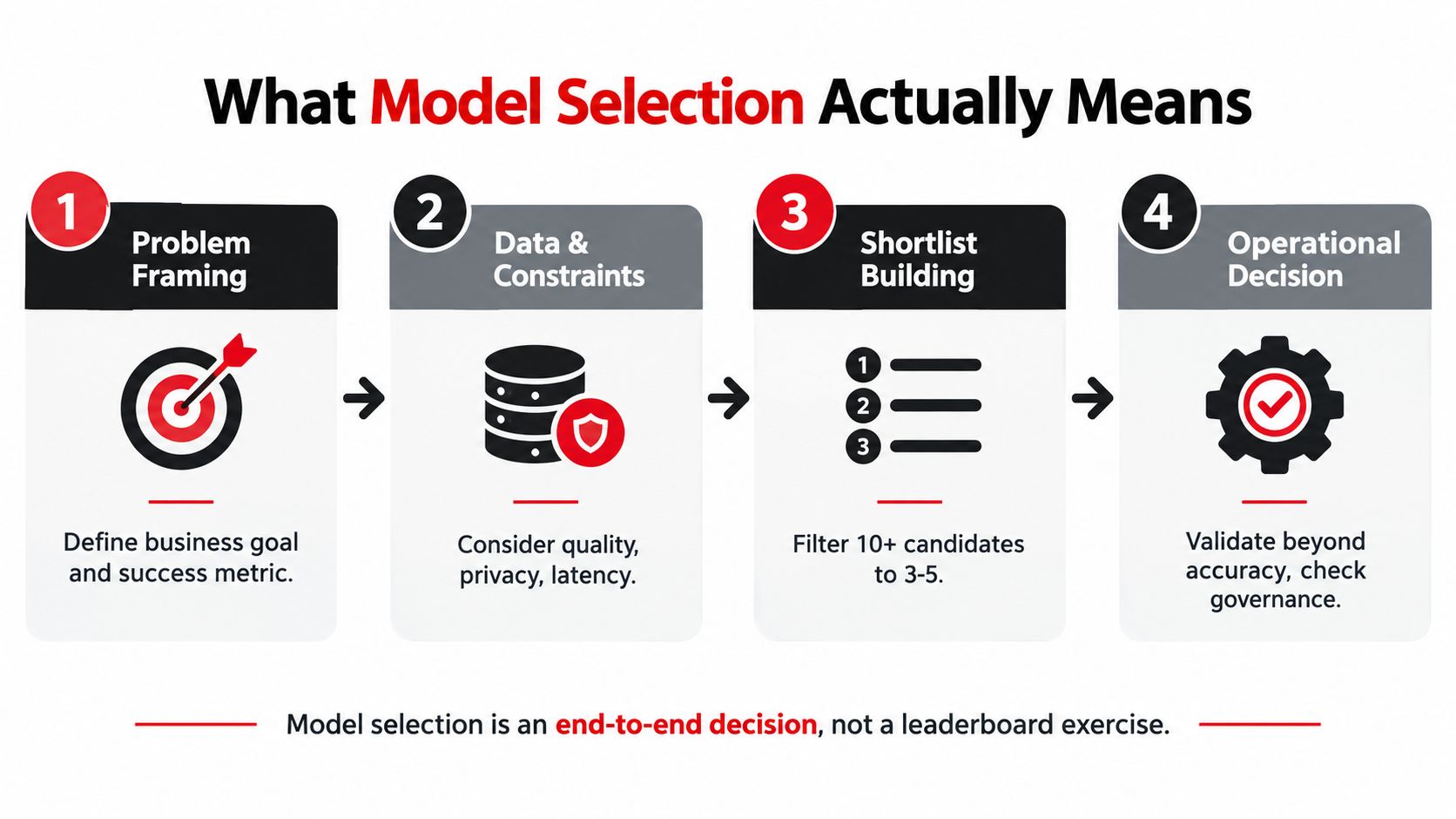
Practical rule: The output of selection should explain both why the winner was chosen and why the alternatives were rejected.
A gradient-boosted tree might win a churn comparison on AUC, yet fail a requirement for transparent reason codes or exceed an inference budget. A regularized logistic model might be the correct choice if stakeholders need stable coefficient direction, simple monitoring, and a clear intervention policy. That isn't accepting a “worse” model. It's optimizing the actual system rather than a leaderboard proxy.
Profiling the Dataset and Scoring Data Quality
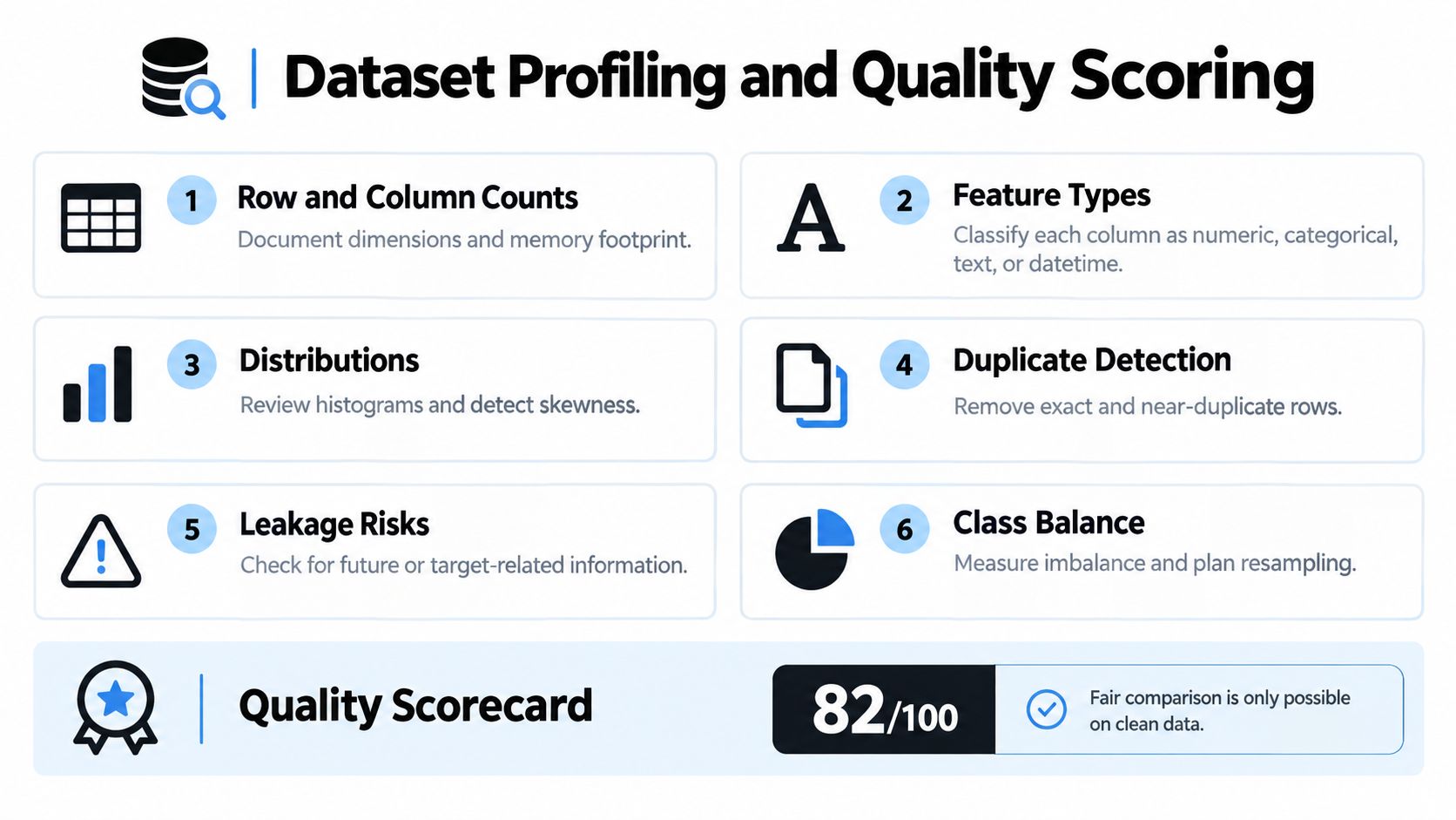
Fair comparison starts with a dataset that candidates receive under the same rules. Profile row and column counts, feature types, distributions, duplicate records, missingness, class balance, and timestamps before fitting models. A high-cardinality categorical variable, near-constant feature, or future-derived timestamp can advantage one algorithm and make the comparison meaningless.
Missingness deserves diagnosis rather than automatic imputation. MCAR means missingness is unrelated to observed and unobserved values, MAR means it can be explained by observed variables, and MNAR means the missingness mechanism depends on unobserved or missing values themselves. The category affects whether ordinary imputation is defensible, whether missingness indicators carry signal, or whether sample-weight adjustments and sensitivity analyses are needed.
Turn profiling into an artifact
An automated profile should flag:
- Completeness: Which columns and rows contain missing values?
- Consistency: Do categories, units, dates, and identifiers follow expected rules?
- Uniqueness: Are duplicate or near-duplicate observations inflating the apparent sample?
- Validity: Do values fall within domain-appropriate ranges?
- Leakage: Does a feature encode the target or information unavailable at prediction time?
- Shift: Do training and holdout distributions differ in ways that affect comparison?
A simple scorecard built from completeness, consistency, uniqueness, and validity gives the team a documented readiness view. It isn't a substitute for domain judgment, but it forces the team to record why the data is considered usable and what limitations remain. The right conclusion may be that cleaning matters more than changing the algorithm.
For a repeatable routine, freeze the raw snapshot, generate the profile, record every exclusion and transformation, create leakage checks, and save the resulting report beside the training configuration. PlotStudio can support this kind of workflow through its data profiling workflow, while keeping the generated Python available for inspection.
Baselines Candidates and Validation Design
A baseline gives every later claim a reference point. Use the simplest predictor that matches the task, such as the majority class, a mean, last-value carry-forward, or logistic regression with a small feature set. If a candidate barely beats that floor, the added maintenance and governance burden may not be justified.
Candidate families should span complexity tiers without becoming an indiscriminate search. For tabular data, compare linear methods with tree ensembles. For text or vision, establish a simple representation and baseline before testing larger neural architectures. For sequential data, use a transparent temporal baseline before introducing recurrent or attention-based systems.
Validation design must follow the data-generating process. Nested cross-validation places hyperparameter tuning and feature decisions in an inner loop, then estimates generalization in an outer loop whose folds weren't used for tuning. This separation is important because the selected minimizer of a finite-variance cross-validation estimate may differ from the model with the lowest true risk, as described in the technical discussion of nested cross-validation.
Keep a final test set untouched until the selection process is complete. Pre-commit the split logic and fold configuration before examining comparative results.
| Data Type | Recommended Scheme | Common Pitfall | Fold Count Guidance |
|---|---|---|---|
| Independent classification | Stratified K-fold | Minority classes disappear from some folds | Pre-commit a fold count that preserves class representation |
| Grouped users or sessions | Grouped K-fold | Records from one entity appear in both training and validation | Keep groups intact |
| Time series | Time-based or rolling split | Future observations influence past predictions | Preserve temporal order |
| Repeated measurements | Subject-level grouped split | The same subject leaks across folds | Split by subject, not row |
| Tuned models | Nested cross-validation | Tuning and reporting reuse the same folds | Separate inner and outer loops |
A validation scheme that flatters every candidate still produces a bad decision. The question isn't whether the winner looks strong under the protocol. It's whether the protocol resembles deployment.
Choosing Metrics That Match the Question
Metrics are the contract between predictions and decisions. A single score compresses distinct failure modes into one ranking, so define a primary metric and at least one guardrail before training. The metric should reflect what happens after the prediction is used, not merely what is easy to calculate.
For imbalanced binary classification, PR-AUC often gives a more decision-relevant view of minority-class retrieval than ROC-AUC. Use F1 when precision and recall have roughly equal importance, or F-beta when you can justify giving one more weight. If predicted probabilities drive prioritization or thresholds, log-loss and Brier score help evaluate calibration rather than ranking alone. The precision and recall trade-off is a decision question, not a cosmetic chart choice.
For multiclass classification, macro-F1 reveals whether the model neglects smaller classes, while micro-F1 reflects aggregate volume. Top-k accuracy is useful when the system only needs to place the correct suggestion within a set of recommendations. For regression, RMSE fits decisions with squared-error penalties, while MAE is easier to interpret when extreme errors shouldn't dominate. MAPE needs caution near zero because its denominator can make the result unstable. Ranking problems commonly call for NDCG or MAP.
| Task | Primary Metric | Secondary or Guardrail | Watch Out For |
|---|---|---|---|
| Imbalanced binary classification | PR-AUC | Recall, precision, calibration | A high ROC-AUC can hide weak minority retrieval |
| Thresholded classification | F1 or F-beta | Precision, recall, Brier score | The threshold changes the operational trade-off |
| Probability forecasting | Log-loss or Brier score | Calibration plots, discrimination metric | Good ranking doesn't guarantee reliable probabilities |
| Multiclass classification | Macro-F1 or micro-F1 | Per-class recall, top-k accuracy | Aggregate scores can hide neglected classes |
| Regression | RMSE or MAE | Error by segment, quantile summaries | MAPE behaves poorly near zero |
| Ranking | NDCG or MAP | Recall at a chosen rank | A global average can hide position-specific failures |
Diagnose the gap instead of worshipping it
Suppose a gradient-boosted model narrowly beats logistic regression. The score tells you that a difference exists under the evaluation design, but not why. Start with slice-by-slice residual and error analysis. For regression, inspect predicted-versus-actual plots, residual-versus-predicted plots, and time-ordered residuals. For classification, examine calibration curves and reliability diagrams.
A probability of 0.8 that is correct only 60 percent of the time is a liability when teams use it to trigger an intervention. Calibration can be improved or assessed separately from ranking, so don't treat raw probabilities as trustworthy merely because AUC is high.
Learning curves help distinguish high bias from high variance. If training and validation error converge as more data arrives, increasing sample size may have limited value and model capacity may be the relevant ceiling. Feature importance and SHAP values can explain direction and contribution, while partial dependence can reveal whether a model learned a plausible relationship or a proxy for an unwanted variable.
End the comparison with a short written diagnosis. Name the dominant failure mode, identify the affected slices, and specify the cheapest experiment that could disprove your explanation.
Balancing Accuracy Interpretability and Latency
Single-objective selection hides decisions inside the metric. A better approach makes the trade-offs explicit with a multi-objective rubric covering predictive quality, interpretability, inference latency, training burden, and governance. You can use weighted scoring, hard constraints, or a Pareto frontier when no candidate dominates across every dimension.
The weights must come from the use case. A regulated churn model may favor logistic regression or a shallow gradient-boosted model because reason codes, reviewability, and stable behavior matter. A low-latency recommender may prefer a distilled model or linear scorer if serving speed and resource limits dominate. A tiny metric advantage isn't automatically worth a substantial increase in p99 latency or a loss of explainability.
| Criterion | Weight | Logistic Regression | Gradient Boosting | Deep Ensemble |
|---|---|---|---|---|
| Predictive performance | Documented by team | Strong baseline | Flexible nonlinear fit | Potentially highly flexible |
| Interpretability | Documented by team | Coefficients and odds direction | Partial dependence and feature attribution | More difficult to explain consistently |
| Inference latency | Documented by team | Usually simple to serve | Depends on tree count and depth | Often operationally heavier |
| Governance fit | Documented by team | Straightforward review | Requires additional controls | Requires stronger documentation |
| Maintenance burden | Documented by team | Low | Moderate | High relative complexity |
The table deliberately uses qualitative entries. Weights are not universal facts, and assigning invented precision to them creates false confidence. Record who selected each criterion, what constraint it represents, and what evidence would cause the weight to change.
Selection should expose disagreement. If one stakeholder optimizes AUC and another optimizes reviewability, put both objectives in the decision record instead of hiding the conflict inside an unexplained score.
Document every rejected candidate. A useful rejection note says that the model failed a latency constraint, had unstable performance on a critical slice, required unavailable features, or offered too little gain for its added complexity. An AI analytics platform can help organize comparative analyses, but the human team still owns the objective function and approval decision.
Hyperparameter Tuning and Automated Selection
Tuning becomes unreliable when the search process is treated as invisible experimentation. Grid search works for a small, low-dimensional space. Random search is a strong default when only some parameters are likely to matter. Bayesian optimization, using tools such as Optuna or Hyperopt, can be useful when each trial is expensive and previous evaluations should guide the next proposal. Population-based methods suit some deep learning workflows with adaptive budgets.
The method matters less than the controls around it. Set a fixed compute budget, use early stopping where appropriate, log every trial, version the configuration, and preserve the data and code references that produced each score. A tuning curve that has flattened is evidence to stop searching, especially when the remaining gains are smaller than the uncertainty in the validation estimate.
Keep automation subordinate to methodology
Nested cross-validation protects the final estimate from the tuning loop. Reusing a finite validation set across repeated searches can overfit the selection criterion itself, a problem demonstrated by Cawley and Talbot's analysis of model-selection overfitting. The practical response is to isolate the final test set, use nested or repeated validation, and treat small gains with skepticism.
The modified one-standard-error rule provides a useful conservative option. It favors a simpler model whose estimated score falls within one standard error of the best candidate, reducing the chance that score noise determines the choice, as discussed in research on regularizing model selection.
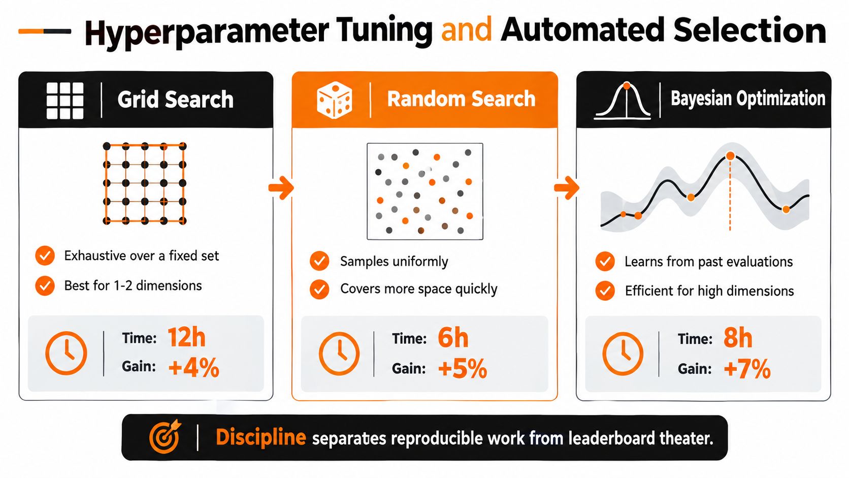
Automation should generate candidates, not erase the rationale.
AutoML and neural architecture search can expand a shortlist, but a black-box winner is difficult to defend if the team can't explain the data preparation, search space, validation procedure, and operational consequences. For changing environments, selection may need to happen repeatedly by segment, query type, or time window. Recent work on active, Pareto, and online selection reflects this shift toward choosing dynamically rather than assuming one model remains best forever, as illustrated by the ICML 2026 session on adaptive model selection.
Deployment Monitoring and Reproducibility
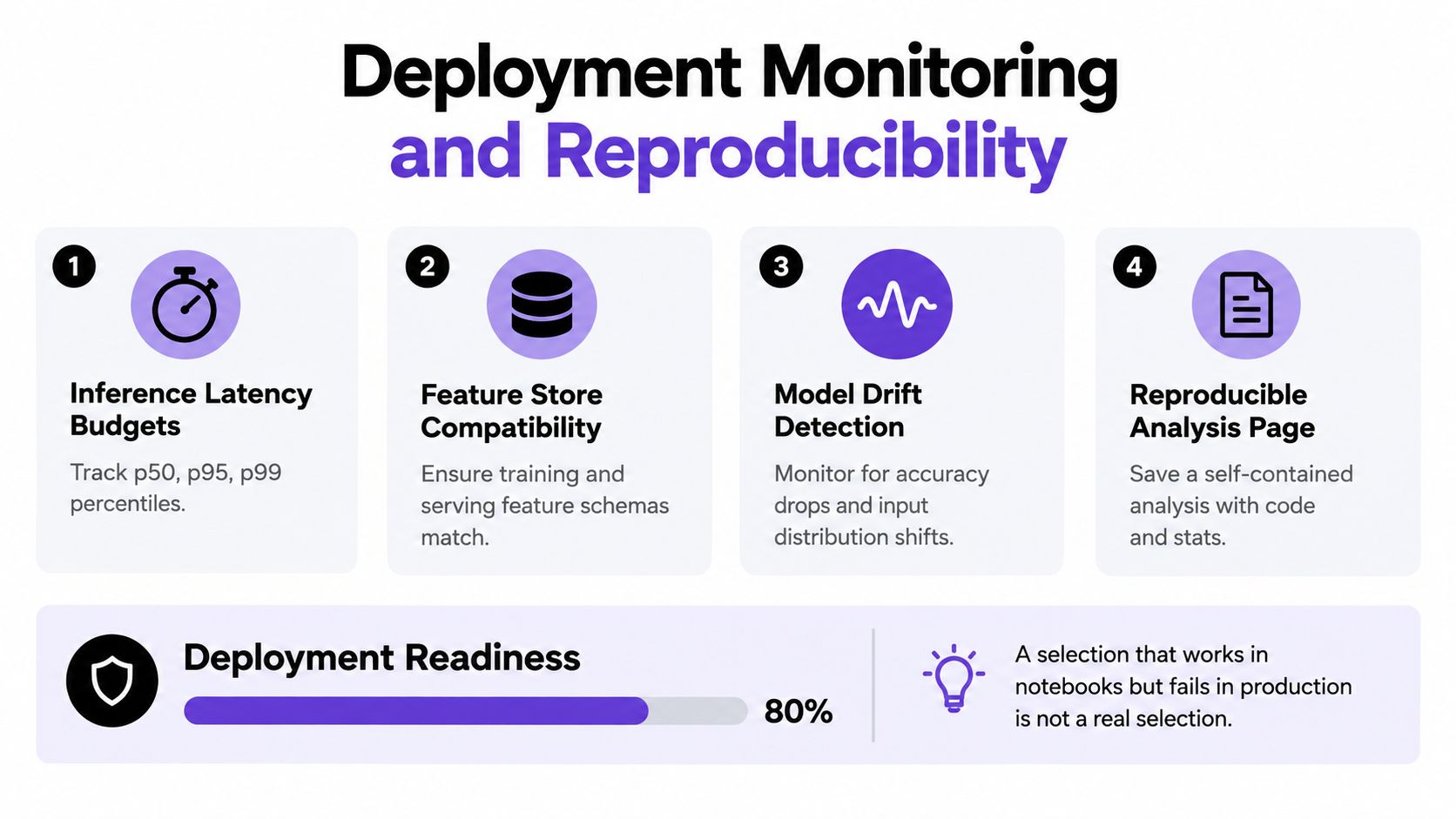
A model that works in a notebook but fails in production wasn't selected successfully. The decision includes inference latency, feature-store compatibility, retraining cadence, drift detection, and the ability to explain and retire the model. Track input distributions, prediction distributions, label availability, and realized performance where labels arrive later.
Common failures include training-serving skew, silent label shift, and concept drift after a policy change. A feature pipeline can produce valid-looking values while changing their meaning, so schema checks alone aren't enough. Monitoring should connect technical signals to business outcomes and define an owner for investigation.
Preserve the rebuild path
Every selected candidate needs a reproducibility manifest containing pinned library versions, a hashed training-data snapshot, configuration files, random seeds, feature definitions, and the exact validation code. Add a model card that states intended use, known limitations, evaluation slices, fairness checks, and conditions under which the model should be retired.
A saved, inspectable research reproducibility workflow makes this standard easier to apply beyond production services. PlotStudio is built around agentic analytics: it plans multi-step work, writes and runs real Python locally, checks its outputs, and saves an Analysis Page with narrative, charts, code, and statistics. That is materially different from chat-with-your-data software, where an answer is a data point and an analysis is often left to the user to reconstruct.
A run-tomorrow checklist
- Frame the problem: Save a problem statement with the prediction unit, action, horizon, loss, and constraints.
- Profile the data: Produce a data quality report covering types, distributions, duplicates, missingness, leakage, and balance.
- Build baselines: Save a baseline notebook and record the assumptions behind each simple predictor.
- Define validation: Create a validation plan with split logic, grouping rules, temporal boundaries, and pre-committed folds.
- Choose metrics: Store a metric table with one primary score and at least one guardrail.
- Diagnose failures: Export residual plots, calibration views, learning curves, and slice-level comparisons.
- Weigh trade-offs: Complete a trade-off matrix covering quality, interpretability, latency, governance, and maintenance.
- Tune carefully: Preserve a tuning log with trial configurations, budgets, stopping rules, and validation results.
- Lock reproducibility: Create a manifest with data hashes, package versions, seeds, code, and model-card details.
- Set monitoring: Define monitoring thresholds, alert owners, retraining triggers, and retirement conditions.
Frequently Asked Questions
How many candidate models should I try?
Try enough candidates to cover the plausible complexity and representation choices for the task, not every algorithm available. A defensible shortlist includes a simple baseline, a strong interpretable candidate, and one or more flexible candidates that address a known limitation. Expand it only when diagnostics show that the current families cannot represent the relevant signal.
Does more data beat a better algorithm?
Sometimes. Learning curves provide the observable test: if validation performance improves meaningfully as the training set grows, more representative data may help. If the curves have converged, investigate feature quality, target definition, leakage, and model capacity before collecting data indiscriminately.
How do I know if I'm overfitting the validation set?
Warning signs include repeated tuning against the same folds, shrinking gains after many trials, unstable rankings across resamples, and a large difference between cross-validated estimates and the final untouched test result. Cawley and Talbot show why the selection process itself can become optimistic when a finite validation set receives repeated feedback, so isolate the test set and use nested validation when tuning is substantial.
When should I stop tuning?
Stop when the tuning curve has flattened, the remaining improvement is smaller than the uncertainty you can resolve, or the candidate has already met the operational requirement. Also stop when a simpler model is within the chosen uncertainty rule and has a clearer governance case. More search isn't automatically more rigor.
Machine learning model selection is complete when the chosen model, validation evidence, operational constraints, and reproducibility artifacts support the same decision. Visit PlotStudio to run local, agentic analytics that turns uploaded data into a planned, executable, inspectable Analysis Page with Python, charts, statistics, and exportable Jupyter or PDF outputs. Use it to make your next selection analysis easier to review without surrendering methodological control.