Stop Reviewer Objections: Missing Data Imputation for Researchers

Imputation replaces missing values with statistically defensible estimates, and the method you choose should follow your analysis goal, not the other way around. For inference, multiple imputation through MICE is the standard because it propagates uncertainty into your final estimates. For prediction, a model with native missing-value handling, like histogram-based gradient boosting, is often a stronger baseline than any imputer you could build. Either way, the missingness mechanism, whether MCAR, MAR, or MNAR, determines whether your chosen approach produces valid results or quietly biased ones.
TL;DR:
- Imputation methods should be chosen based on analysis goals, with multiple imputation preferred for inference and native model handling for prediction tasks.
- Diagnosing the missingness mechanism (MCAR, MAR, MNAR) is crucial, with visual and statistical checks guiding appropriate handling and sensitivity analysis for MNAR cases.
- Imputation policies must involve training on only training data, scaling variables beforehand, and recording parameters to ensure reproducibility and prevent data leakage.
- Multiple imputation with Rubin’s rules provides more honest uncertainty estimates, especially when missingness exceeds 10%, and should be accompanied by distributional and convergence diagnostics.
- Neural network-based imputers are useful for complex data but are often unnecessary for tabular data with fewer samples, making classical methods like MICE more practical for most research.
Table of Contents
- What Missing Data Imputation Actually Requires You to Diagnose First
- A Decision Framework for Imputing, Dropping, or Letting the Model Handle It
- Common Imputation Methods, From Simple Fills to Multivariate Models
- Building an Implementation Pipeline That Won’t Leak or Break on Rerun
- Measuring Whether Your Imputations Actually Hold Up
- When MNAR Breaks the Rules and How to Report It Honestly
- How Plotstudio Supports Reproducible, Auditable Imputation Workflows
- Handling Missing Data in Time Series
- Imputation Challenges With High-Dimensional Data
- The Impact of Imputation on Downstream Analysis and Modeling
- Advanced Imputation Methods Using Deep Learning and Neural Networks
- Author Perspective: A Pragmatic Checklist Before You Submit
- Try a Reproducible Imputation Workflow With Plotstudio
- Sources
- FAQ
What Missing Data Imputation Actually Requires You to Diagnose First
Every imputation decision rests on a question that’s easy to skip and expensive to ignore: why is the data missing? Statisticians sort missingness into three mechanisms, and getting this classification wrong doesn’t just cost you elegance. It can invalidate your entire downstream analysis.
Missing Completely at Random (MCAR) means the probability of a value being missing has nothing to do with any variable, observed or not. A sensor that randomly drops readings due to a hardware glitch is a clean MCAR example. Under MCAR, a complete-case analysis is unbiased, though it wastes statistical power.
Missing at Random (MAR) means missingness depends on observed variables but not on the missing value itself. Suppose income is missing more often for younger survey respondents. If age is recorded, you can model that pattern and impute accurately, because the “randomness” is conditional on something you can see.
Missing Not at Random (MNAR) is the hard case. Missingness depends on the unobserved value itself. High earners who decline to report income, or patients who drop out of a trial specifically because a treatment isn’t working, are classic MNAR patterns. This is the scenario where most standard imputers, including MICE, quietly fail unless you build in explicit corrections.
This mechanism classification governs whether imputation can produce unbiased results at all, according to a detailed review of missing data handling published in PMC. Treating imputation as a preprocessing checkbox rather than a design decision is one of the most common mistakes in applied research.
How to diagnose the mechanism in practice
You can’t always prove a mechanism definitively, but you can gather strong evidence with a few standard checks:
- Missingness matrices. Visualize which variables are missing together. Correlated missingness patterns (e.g., income and employer name always missing together) hint at a shared underlying cause.
- Pairwise group comparisons. Split your dataset into “missing” and “observed” groups for a variable, then compare means or distributions of other observed variables between them. Large differences suggest MAR rather than MCAR.
- Logistic regression on missingness. Fit a model predicting whether a value is missing (1/0) using other observed features. Significant predictors indicate MAR; a null model is consistent with MCAR.
- Little’s MCAR test. A formal statistical test, though it has limited power in small samples and should be paired with the visual checks above rather than used alone.
- Simulation-based diagnostics. Synthetic experiments comparing MCAR and MAR dropout illustrate the risk directly. Simulations run on real datasets show that dropping observations under MAR skews the resulting distribution, while MCAR samples remain representative, according to an applied walkthrough on handling missing data.
The uncomfortable truth is that MNAR can rarely be confirmed or ruled out from the data alone, since it depends on the very values you don’t have. When you can’t determine the mechanism with confidence, the correct move isn’t to guess. It’s to run sensitivity analyses under a few plausible MNAR scenarios and report how much your conclusions shift. If your effect size survives a range of reasonable assumptions, you have a much stronger paper than one that silently assumes MCAR and hopes nobody asks.
A Decision Framework for Imputing, Dropping, or Letting the Model Handle It
Before writing a line of imputation code, run through a short checklist. It takes ten minutes and prevents the single most common reviewer objection: an imputation choice with no stated rationale.
- State your analysis goal. Are you estimating a population parameter (inference) or building a model that predicts new cases (prediction)? This single answer determines almost everything downstream.
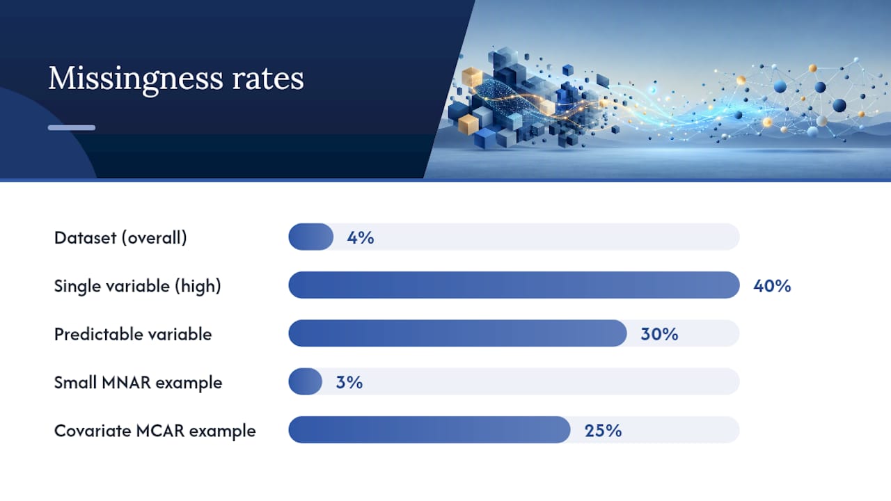
- Check missing rate per variable, not just overall. A dataset that’s 4% missing in aggregate can hide one variable that’s 40% missing. Report rates variable by variable.
- Check correlation with other observed features. A variable with 30% missingness that’s highly predictable from three other columns is a much safer imputation candidate than one that’s missing at random with no useful predictors.
- Weigh importance to the core finding. If a variable is central to your hypothesis, invest more care (multiple imputation, sensitivity analysis) than you would for a peripheral covariate.
- Consider your sample size. Small samples amplify the variance-understatement problem of single imputation methods, making multiple imputation more important, not less.
Ignore the popular “5% missing data rule,” the rough heuristic claiming that anything under 5% missingness can be safely ignored or mean-imputed without consequence. It isn’t grounded in any statistical theory that accounts for mechanism, variable importance, or correlation structure. A variable with 3% MNAR missingness tied directly to your outcome can bias a result more than a variable with 25% MCAR missingness in a covariate nobody cares about. Percentage thresholds ignore the question that actually matters: why is this value missing, and does that reason correlate with what you’re trying to measure?
Adding a missingness indicator, a binary flag marking which rows were originally missing, is worth doing whenever you suspect the missingness itself carries information (MAR or MNAR patterns). Skip it and rely on a structural constant instead when missingness reflects a genuine “not applicable” case, like a “years married” field that’s legitimately blank for single respondents.
Pro Tip: Run your decision checklist twice: once before you look at the missingness patterns, and once after. If your planned approach changes after seeing the data, document why. That’s exactly the kind of transparency a peer reviewer wants to see in your methods section.
Common Imputation Methods, From Simple Fills to Multivariate Models
Method choice separates a defensible paper from one that gets a “methods insufficiently justified” note from a reviewer. Here’s how the standard toolkit breaks down.
Simple univariate methods (mean, median, mode, or a constant) fill every missing value in a column with a single computed statistic. They’re fast and numerically stable, which is why they remain common as a quick baseline. The cost is real: they systematically understate variance, since every imputed value is identical, and they can distort correlations between variables. Scikit-learn’s SimpleImputer implements this cleanly for cases where speed matters more than precision, according to the scikit-learn imputation documentation.
KNNImputer fills a missing value using the average (or weighted average) of the k nearest neighboring rows, measured across the other observed features. It captures local structure that a global mean can’t, but it’s sensitive to feature scale. A distance calculation on unscaled data lets a variable measured in the thousands dominate one measured in decimals. The n_neighbors parameter is a real trade-off: smaller values pick up local structure but add noise, while larger values smooth things out and lean toward the simple-mean behavior you were trying to avoid.
IterativeImputer, scikit-learn’s implementation of the MICE idea, models each feature with missing values as a function of all other features, in a round-robin fashion, cycling through variables until estimates stabilize. This is fundamentally different from a single deterministic fill. Run with sample_posterior=True, it draws from the conditional posterior distribution rather than just predicting the mean, which is what makes true multiple imputation possible: generate several completed datasets, each with slightly different plausible values, and combine the results afterward.
Predictive mean matching (PMM) is a refinement worth knowing even if you don’t implement it from scratch. Rather than plugging in a regression’s predicted value directly, PMM finds real observed values close to that prediction and imputes one of those. This keeps imputed values within the realistic range of the data. It’s why PMM is often preferred over raw regression imputation in fields like clinical research, where an imputed lab value should look like a lab value that could plausibly exist.
Hot-deck imputation, borrowing an actual observed value from a similar respondent rather than a model-generated estimate, plays a similar role in survey statistics, preserving the natural distribution of the data at the cost of some added implementation complexity.
Model-native missing handling deserves a place in this comparison, not as an imputation method, but as an alternative to imputing at all. Histogram-based gradient boosting models can route missing values down a learned split direction during training, without any preprocessing step. This is worth trying as a baseline before you build out a full imputation pipeline, particularly for prediction tasks where inferential validity isn’t the goal.
Here’s how these methods stack up against each other:
| Method | Best for | Computational cost | Preserves uncertainty | Ease of implementation | Sensitivity to scaling |
|---|---|---|---|---|---|
| Mean/median/mode | Quick baselines, large low-stakes datasets | Very low | No | Very easy | None |
| KNNImputer | Small to mid-size datasets with local structure | Moderate | No (single fill) | Easy | High |
| IterativeImputer (single) | Multivariate structure, moderate size | High | No (single fill) | Moderate | High |
| MICE (multiple imputation) | Inferential analyses, papers, grants | High | Yes | Moderate to hard | High |
| Native missing handling (histogram GBM) | Prediction tasks, high missing volume | Low | Not applicable | Very easy | None |
Method selection correlates strongly with dataset size. Scikit-learn’s own comparisons show IterativeImputer often outperforming mean imputation on small datasets, while on large datasets mean imputation can perform comparably at a fraction of the compute cost, based on scikit-learn’s imputation benchmark examples. That’s a genuinely counterintuitive finding worth internalizing: more sophistication doesn’t always buy you more accuracy, and knowing when it doesn’t can save you hours of runtime on a dataset with a million rows.
Building an Implementation Pipeline That Won’t Leak or Break on Rerun
The gap between “the imputation math is correct” and “the imputation pipeline is reproducible” is where most defensibility problems actually live. Follow these rules in order.
- Fit imputers on training folds only. Any statistic computed for imputation, means, regression coefficients, nearest-neighbor distances, must come exclusively from training data. Wrap the entire sequence in a scikit-learn
Pipelineso cross-validation automatically refits the imputer inside each fold rather than leaking test-set information into your fill values. - Scale before distance-based or regression-based imputation.
KNNImputerandIterativeImputerboth operate on feature magnitude, so unscaled variables distort results. A walkthrough on multivariate imputation recommends scaling before running either method, and suggestsRobustScalerspecifically when your features have long tails or outliers, since it centers on the median rather than the mean. - Set
add_indicator=Truewhenever missingness itself might carry signal. This appends a binary “was this value missing” column alongside the imputed feature, letting downstream models learn from the missingness pattern directly rather than losing that information at the imputation step. - Handle categorical variables carefully. Decide whether to encode before or after imputation, and be cautious with target-guided encoding schemes (ordering categories by their relationship to the outcome) applied before imputation, since this can leak outcome information into your fill values.
- Record your seeds and imputer versions.
IterativeImputerinvolves randomness in its regression steps. Storerandom_state, the scikit-learn version, and your key parameters (max_iter,tol,n_nearest_features,skip_complete) in your methods section or a version-controlled config file.
On that last point: n_nearest_features limits how many other columns each feature’s imputation model considers, which matters a great deal once you have dozens of correlated predictors and don’t want every regression step conditioning on all of them. skip_complete=True tells the imputer to leave fully observed columns untouched during the iterative rounds, saving compute. max_iter and tol control how many round-robin cycles run before the algorithm calls it converged, according to the scikit-learn documentation.
Pro Tip: Persist your fitted imputer object (via joblib or pickle) alongside your saved model. If a reviewer or collaborator asks you to reproduce a result on new data eighteen months later, refitting the imputer from scratch on a slightly different data snapshot can shift your results in ways nobody can explain after the fact.
Measuring Whether Your Imputations Actually Hold Up
A single imputed dataset, no matter how sophisticated the method, understates the true uncertainty in your estimates, because it treats a guess as if it were observed fact. Multiple imputation solves this by generating several completed datasets, each with independently drawn plausible values for the missing cells, then running your analysis on each one separately.
The results are combined using Rubin’s rules, a set of formulas that pool the point estimates by simple averaging and combine the variance from two sources: the average within-imputation variance, and the between-imputation variance that captures how much your estimates disagreed across the different completed datasets. This second term is exactly what single imputation throws away, and it’s why properly pooled multiple-imputation confidence intervals are almost always wider, and more honest, than the ones you’d get from a single mean-filled dataset. This approach is the standard recommendation for inferential work, according to a tutorial on multiple imputation in clinical research.
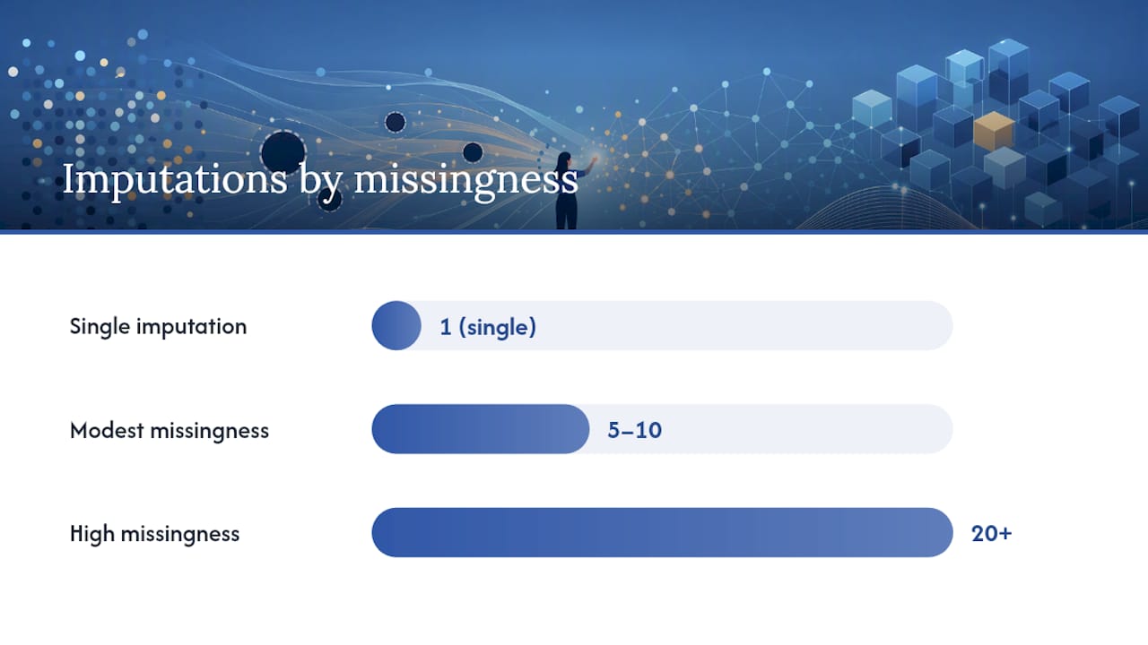
How many imputations, M, do you need? There’s no rigid universal number. A practical guideline is to scale M with your missing data fraction. Datasets with modest missingness (under 10%) often do fine with 5 to 10 imputations, while higher missingness rates or analyses sensitive to small estimate shifts benefit from 20 or more. Running M at a level too low to stabilize your pooled variance estimate is a common, quietly damaging shortcut.
Beyond the pooling mechanics, a few diagnostics belong in every imputation-based analysis:
- Distributional checks. Overlay the distribution of imputed values against observed values for the same variable. Wildly different shapes are a red flag.
- Convergence checks. For
IterativeImputer, confirm that successive iterations stabilize rather than oscillating, particularly withsample_posterior=True. - Sensitivity analyses under alternative MNAR assumptions. Re-run key analyses under a few plausible “what if the missingness depended on the outcome” scenarios and report how much conclusions move.
- End-to-end cross-validation. For predictive work, cross-validate the entire pipeline, imputer included, and compare against a model-native missing-handling baseline. If a histogram-based gradient boosting model with no imputation step matches your carefully imputed pipeline’s performance, that’s worth reporting.
When MNAR Breaks the Rules and How to Report It Honestly
Standard imputers, including MICE, assume the missingness mechanism is at least MAR. Under true MNAR, where the probability of missingness depends on the unobserved value itself, that assumption fails, and no amount of additional predictors in your imputation model fixes it, because the very thing driving the missingness isn’t in your dataset.
Two formal strategies exist for this situation, though both require assumptions you can’t fully verify from the data:
- Selection models jointly model the outcome and the missingness mechanism, assuming a specific relationship between them (commonly a Beckman-style correction). They’re powerful but fragile, since results hinge heavily on the assumed selection equation.
- Pattern-mixture models stratify the analysis by missingness pattern and model each stratum separately, then combine results under explicit assumptions about how the missing and observed groups differ.
- Sensitivity analyses are the pragmatic middle ground favored in most applied papers: rather than committing to one MNAR model, you test how conclusions shift under a range of plausible assumptions and report the results as a supplementary table.
Structural missingness, where a value is blank because the question genuinely doesn’t apply, deserves different treatment entirely. Coding “not applicable” as a domain-meaningful constant, rather than imputing it as if it were a random gap, is usually more honest than any statistical fill. Pair that constant with an explicit indicator column so downstream models and readers can distinguish “structurally not applicable” from “randomly missing.”
Sometimes computational or sample-size constraints genuinely justify a simpler method than the theory would prefer. That’s fine, but say so plainly in your limitations section rather than letting a reviewer discover it. A single sentence like “given a sample size of 84, we used median imputation rather than multiple imputation to avoid overfitting the imputation model itself” is far stronger than silence.
How Plotstudio Supports Reproducible, Auditable Imputation Workflows
Everything covered so far, mechanism diagnosis, method selection, pipeline hygiene, uncertainty propagation, has to survive contact with a reviewer, a supervisor, or an IRB audit eighteen months after you ran it. That’s the actual bar for research-grade imputation, and it’s the problem Plotstudio is built around.
An agentic analytics platform can support academic research by producing results defensible enough for papers, theses, grant applications, and peer review, not just quick exploratory charts.
- Analysis runs locally on your own machine. Your dataset never leaves the device, which matters directly for IRB-governed data, NHS records, or GDPR special-category patient information that institutional policy often prohibits uploading to a cloud tool.
- Every analysis is gated behind a reviewable, approvable plan. Before any code executes, you see the stated method, assumptions, and success criteria, functioning as a pre-registration step and an audit trail you can point a reviewer to directly.
- Skills encode your field’s methodology once. A lab can define required diagnostic steps, statistical thresholds, and forbidden shortcuts for imputation, so every subsequent analysis follows that standard rather than a generic default.
Pre-registering your imputation approach and archiving the resulting artifacts strengthens a paper’s defensibility considerably, a point echoed in broader guidance on missing data best practices. Some tools export annotated notebooks and PDF reports alongside permanent, searchable analysis pages, facilitating detailed methods documentation and reproducibility.
Handling Missing Data in Time Series
Time series data breaks the independence assumption most imputation methods quietly rely on. A missing temperature reading at 3 p.m. is not just “a missing value.” It’s flanked by readings at 2 p.m. and 4 p.m. that carry strong information about it, and treating it like an independent MCAR gap wastes that structure entirely.
Linear interpolation is the simplest reasonable default for short gaps in smoothly trending series. For seasonal data, seasonal decomposition-based imputation, filling gaps using the seasonal and trend components separately, tends to outperform a flat interpolation across a holiday spike or a weekly cycle. Longer gaps call for model-based approaches: state-space models like Kalman smoothing handle irregular gaps well and naturally produce uncertainty estimates alongside the fill, which matters if you’re propagating that uncertainty into a downstream forecast.
The mechanism question still applies, with a time series twist. A sensor failure is closer to MCAR. A stock-price series missing on days markets are closed is structural, not random, and should be coded as such rather than imputed at all. Gaps caused by a bond trader manually pulling volatile data points before a report, if that ever happened, would be MNAR, and no amount of interpolation fixes that kind of gap. Always check whether your missingness clusters around specific dates, events, or regimes before choosing a method, since clustered gaps are rarely MCAR.
Imputation Challenges With High-Dimensional Data
As the number of features grows, IterativeImputer’s round-robin regression approach gets expensive fast, since it fits a separate model for every incomplete column, conditioned on every other column, each iteration. On a dataset with hundreds of variables, this can turn a minutes-long job into an hours-long one.
The n_nearest_features parameter exists specifically for this problem, limiting each column’s imputation model to its most correlated neighbors rather than the full feature set, according to the scikit-learn documentation. This keeps runtime manageable without abandoning the multivariate approach entirely.
High dimensionality also amplifies a subtler problem: with many correlated predictors, small imputation errors in one column can propagate and compound across the others during the iterative fitting process, especially if convergence is loose. Tightening tol and increasing max_iter helps, at the cost of runtime.
Dimensionality reduction before imputation, such as imputing on a reduced set of principal components and projecting back, is one workaround worth testing, though it adds a layer of complexity to your reporting that needs its own justification in the methods section. For genuinely high-dimensional settings (hundreds to thousands of features), a pragmatic move many researchers underuse is testing whether a model-native handling approach, like histogram-based gradient boosting, matches your imputation pipeline’s performance at a fraction of the setup cost. If it does, you’ve saved yourself a defensibility headache for no accuracy loss.
The Impact of Imputation on Downstream Analysis and Modeling
Imputation choice isn’t a preprocessing footnote. It changes point estimates, standard errors, and sometimes the direction of a reported effect, which is exactly why a reviewer will ask about it if you don’t address it first.
For inferential work, single imputation methods, mean fill especially, systematically shrink standard errors because every imputed value is treated as if it were known with certainty. This can turn a genuinely uncertain finding into one that looks artificially significant. Multiple imputation, pooled with Rubin’s rules, corrects this by folding the between-imputation disagreement into your final variance estimate, typically widening confidence intervals compared to a naive single fill.
For predictive modeling, the impact shows up differently: in feature importance and generalization. An imputed feature that leaked information from the full dataset (rather than being fit strictly on training folds) will look artificially predictive during training and then underperform on genuinely new data. This is precisely the leakage problem a proper pipeline structure prevents. It’s also worth directly comparing your imputed pipeline’s cross-validated performance against a model-native missing-handling baseline. If the baseline wins or ties, your imputation step was adding complexity without adding value.
The honest move, in either case, is reporting results with and without your chosen imputation approach, or across a couple of alternative methods, so a reader can see how sensitive your conclusion actually is to that one preprocessing choice.
Advanced Imputation Methods Using Deep Learning and Neural Networks
Neural network-based imputers have moved from research curiosity to genuinely practical tools for specific data shapes, though they come with real trade-offs against the classical methods covered earlier.
Denoising autoencoders learn a compressed representation of your data by training on artificially corrupted (masked) versions of complete rows, then reconstructing the original. Applied to imputation, the trained network fills genuinely missing values using that learned reconstruction. This works especially well on data with strong nonlinear feature interactions that a linear regression-based MICE model would miss.
Generative Adversarial Imputation Networks (GAIN) extend the GAN framework to imputation directly: a generator network fills in missing values, and a discriminator network tries to distinguish which values were originally observed versus generated, pushing the generator toward increasingly realistic fills.
Variational autoencoders (VAEs) offer a probabilistic advantage similar in spirit to MICE’s sample_posterior option: rather than a single deterministic fill, they can sample multiple plausible completions from a learned latent distribution, enabling a neural-network flavor of multiple imputation.
These methods can outperform classical approaches on large, complex datasets with intricate feature dependencies, images, genomic data, or dense sensor arrays being typical use cases. The cost is real: they need substantially more data to train reliably, are harder to explain in a methods section, and introduce their own hyperparameter and convergence diagnostics on top of everything already required for a defensible imputation writeup. For most tabular research datasets, particularly anything under a few thousand rows, the added complexity rarely pays for itself over a well-implemented MICE pipeline.
Author Perspective: A Pragmatic Checklist Before You Submit
Five rules keep an imputation section out of reviewer crosshairs. State your method by name and package version. Report your diagnostics for the missingness mechanism, not just an assumption. State M, the number of imputations, and why you chose it. Record your seeds. Run at least one sensitivity analysis and report it, even briefly.
The reviewer criticisms that recur most often aren’t about method sophistication. They’re about missing detail: no imputer version number, no stated M, no sensitivity check under an alternative mechanism assumption. Put the heavy diagnostics, convergence plots, distributional comparisons, alternative-scenario results, in a supplement rather than the main text, and phrase limitations plainly: “we assumed MAR based on X diagnostic; results under a plausible MNAR scenario are in Supplement B.” That single sentence does more for your credibility than another paragraph of confident-sounding methodology.
— Aymen
Try a Reproducible Imputation Workflow With Plotstudio
If you’ve read this far, you already know the gap between “ran an imputer” and “can defend that imputer to a reviewer eighteen months from now.” Certain analytics platforms aim to support reproducible and auditable imputation workflows by running analysis plans locally on the user’s machine, with documented parameters and pre-execution review steps.

That approval step becomes your pre-registration record. Local execution ensures sensitive data governed by IRB or GDPR special-category regulations can be analyzed without leaving the user’s device. And every run exports as an annotated notebook and PDF report on a permanent, searchable page, exactly the artifact trail a supervisor or reviewer will ask for. Academic researchers can review the Bring Your Own Key academic plan built around institutional needs, while individual researchers and labs evaluating a broader fit can check current pricing and trial options, including the Managed Credits and Bring Your Own Key monthly plans. Start with the free trial and run your next imputation decision through a workflow built to survive peer review.
Sources
- Handling missing data: guidance and review (PMC11101000)
- Imputation of missing values — scikit-learn documentation
- Deal with missingness like a pro: multivariate and iterative imputation algorithms — Towards Data Science
FAQ
What Does Imputation of Missing Data Mean?
Imputation means replacing a missing value in a dataset with an estimated value, generated from a statistical model or rule, so the dataset can be analysed without dropping incomplete rows.
How Much Missingness Is Acceptable?
There’s no safe universal threshold. A variable’s acceptable missing rate depends on its mechanism (MCAR versus MAR versus MNAR), its correlation with other observed features, and how central it is to your core finding, not on a fixed percentage.
What Is the 5% Missing Data Rule?
The 5% rule is an informal heuristic claiming that missingness under 5% can be safely mean-imputed or ignored. It has no grounding in mechanism theory and can mislead you if that small fraction of missing values is MNAR and tied directly to your outcome.
What Are the Three Types of Missing Data?
The three recognized mechanisms are MCAR (missing completely at random), MAR (missing at random, conditional on observed variables), and MNAR (missing not at random, dependent on the unobserved value itself), as detailed in the PMC review on missing data handling.