Multinomial Logit Models Explained

Multinomial logit models estimate the probability that someone picks one option from three or more categories that have no natural order. They're the right call for choices like transport mode, brand preference, or treatment selection—situations where the options are distinct but not ranked. PlotStudio AI supports this kind of research data analysis with reproducible Python analysis, not a single chat response that disappears when the tab closes.

Understanding Multinomial Logit Models

Picture the model as giving every available option a hidden utility score, then turning those scores into probabilities. A higher score nudges the odds in that option's favor, but it doesn't lock in the outcome. That's what makes multinomial logit so useful for studying real-world decisions—it captures the logic of choice while leaving room for the uncertainty that always exists in human behavior.

The method fits when:

• The outcome you're trying to predict is nominal—categories, not numbers or ranks.
• There are three or more possible outcomes, not just yes-or-no.
• Your predictors describe the person making the choice: age, income, education, and so on.
• The categories are clearly different from each other but don't line up on any scale.

Take a transportation study. You might model whether a commuter drives, takes the bus, or cycles. A health researcher could look at which of three therapies a patient prefers. That said, if travel time or cost varies by option, a basic multinomial model may not cut it—you'd want to explore conditional or mixed logit instead. More on those variants shortly.

An answer is an output; an analysis is an investigation. Before you treat any model result as evidence, check the assumptions, compare alternative specifications, and inspect the predicted probabilities.

Choosing the Right Logit Model

The distinction between logit model types comes down to outcome structure, not how many predictors you have. Using ordinal logit when your categories lack order is a common mistake. So is defaulting to binary logit when you have multiple options—that throws away information you paid to collect. If you want a broader refresher on the family, read this guide to logistic regression.

Model Type	Outcome Structure	Key Assumption	Best Use Case
Multinomial logit	Three or more unordered categories	Independence of irrelevant alternatives	Party preference, transport choice, or treatment selection
Binary logit	Two categories	Log-odds change linearly with predictors	Adoption versus non-adoption
Ordinal logit	Ordered categories	Proportional odds across thresholds	Low, medium, or high satisfaction

Picking the wrong model type doesn't just hurt accuracy—it can flip your conclusions. Match the structure first, then worry about predictors.

PlotStudio AI can inspect your categorical data, plan a fitting analysis, run Python locally, and keep your code, diagnostics, charts, and interpretation together in a single Analysis Page. But the judgment call—whether the categories, the assumptions, and the research question actually justify multinomial logit—still rests with you.

Multinomial logit models became a practical framework for studying decisions among several unordered options through a series of statistical and economic breakthroughs. Cox in 1966 and Theil in 1969 laid essential groundwork, and Daniel McFadden's 1973 formulation tied the model to random utility theory and Luce's choice axiom in a way that changed how researchers think about discrete decisions.

That lineage still matters. It explains why the model stays so common across economics, transportation, marketing, and the social sciences — and it reminds practitioners that they're not just fitting a convenient classifier. They're specifying a behavioral story about how a person weighs the unobserved appeal of each available option.

From Utility to Choice Probabilities

Picture a commuter picking between car, bus, and train. Each alternative carries a utility the researcher can't observe directly, shaped by things like income, travel time, and cost. The commuter selects whichever option delivers the highest realized utility, and everything else — the mood they're in, a vague preference for open windows — gets folded into a random error term.

The multinomial logit framework turns those utility differences into choice probabilities through exponentiation:

[
P_{ij}=\frac{\exp(V_{ij})}{\sum_{k=1}^{J}\exp(V_{ik})}
]

Here, (V_{ij}) represents the systematic component of utility for person (i) and alternative (j). Because only relative utility drives the choice, one category typically serves as the reference. That closed-form probability is what makes estimation tractable even when you're working with thousands of observations across dozens of alternatives.

The model's real power is connecting individual decisions to aggregate outcomes. Latent utilities at the person level translate into predicted ridership, brand shares, treatment preferences, or policy adoption rates.

Luce's choice axiom gives the behavioral logic: the relative odds of choosing one option over another depend only on those two options, not on what else sits on the table. That clean implication is also the model's most scrutinized weakness — it's the independence of irrelevant alternatives assumption, and it gets tested hard in applied work.

Why the Foundations Still Matter

Historical theory isn't just academic decoration. It helps researchers defend model choices during specification and peer review — explaining why certain predictors belong, why a reference category is necessary, and when a more flexible nested or mixed logit formulation might be worth the added complexity.

Consider how different types of variables fit. Chooser-specific variables like age and income slide naturally into a standard multinomial logit. But alternative-specific attributes — the travel time for each route, the price of each product — often push researchers toward conditional or mixed logit specifications.

A sound workflow should therefore:

1. Define the choice set and outcome structure clearly.
2. Map each predictor to either the chooser or the alternative.
3. State the utility assumptions explicitly.
4. Test whether the specification actually fits the observed decisions.

For broader context, learn more about econometric analysis and its research applications.

PlotStudio AI can support this kind of investigation by inspecting data, generating Python, testing specifications, and preserving the methodology in an Analysis Page. Its agentic analytics workflow plans out multiple analytical steps and inspects intermediate outputs along the way — though the researcher still needs to decide whether the theoretical assumptions line up with the substance of the question at hand.

The independence of irrelevant alternatives (IIA) says that the odds of picking one option over another stay fixed, even when a third option shows up. That restriction keeps multinomial logit models lean and fast, but it can also misrepresent behavior when two alternatives feel like near-clones to the decision-maker. Treat IIA as a testable assumption, not a free pass.

The diagram below traces the intellectual lineage behind multinomial logit models — from early probability work through to modern choice modeling.

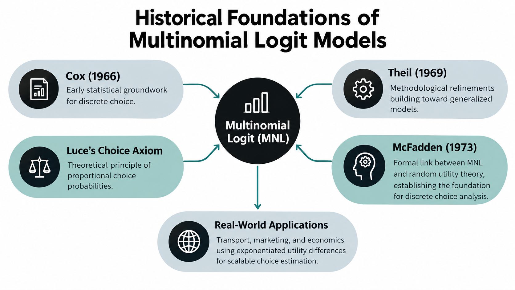
You can see how Cox, Theil, Luce, and McFadden built pieces of a framework now used daily in transport, marketing, and economics. The same map also hints at why the model stays mathematically tractable: it inherits a strong behavioral assumption about how people compare options.

Why IIA Can Distort Substitution

Picture a commuter choosing between car and rail. Now add a bus route that's nearly identical to the existing rail option. IIA insists the new bus steals riders from car and rail in proportion to their original odds. Reality looks different: the bus probably pulls mainly from rail, barely touching car choice.

Economists call this the red bus and blue bus problem. Two buses painted different colors are functionally the same. Adding a second bus should slice the original bus market, not drain demand evenly from trains and cars alike.

IIA isn't claiming new options don't matter. It's claiming the relative odds between any two existing options stay the same, regardless of what else is available.

That assumption holds up well when alternatives are genuinely distinct — say, driving versus flying versus taking a train across a long distance. It gets shaky when options share unobserved qualities like comfort, brand identity, clinical purpose, or convenience.

Before committing to a multinomial logit specification, work through these questions:

• Are some alternatives close substitutes in the eyes of the decision-maker?
• Could unmeasured preferences cluster within groups of options?
• Does adding or dropping an alternative produce plausible predicted changes?
• Does your data include repeated choices from the same individual?

For broader methodological context, see this guide to advanced statistical methods.

Test IIA Before Choosing a Specification

The go-to diagnostic is the Hausman-McFadden test. The logic is straightforward: estimate the full multinomial logit, drop one alternative, re-estimate the restricted version, and compare the coefficient vectors.

A meaningful difference suggests removing that alternative shifts the estimated relationships among the ones left behind — which contradicts IIA. Still, the test isn't a mechanical verdict. Numerical instability, sparse categories, small samples, or poorly behaved covariance matrices can produce misleading outcomes.

A practical workflow looks like this:

1. Fit the planned multinomial logit with a clearly documented reference category.
2. Re-estimate after removing plausible alternative subsets.
3. Compare coefficients, standard errors, predicted probabilities, and substantive conclusions side by side.
4. Check whether the test result stems from data quirks rather than genuine substitution patterns.
5. Bring theory and domain knowledge into the decision alongside the formal test.

A non-significant result supports sticking with the simpler model — but it doesn't prove IIA holds in reality. A significant result tells you it's worth exploring a more flexible specification seriously.

With PlotStudio AI, you can run these comparisons through local Python execution, keep the generated code, and assemble model outputs with diagnostic reasoning on a reproducible Analysis Page. The researcher still weighs the evidence and decides whether the model needs to change.

Choose a Flexible Alternative When Needed

When alternatives naturally group together, nested logit lets you model stronger substitution within clusters — say, bus and rail both sitting inside a "public transit" nest. When preferences differ widely across people, mixed logit introduces random coefficients and captures unobserved heterogeneity.

Conditional logit fits when your predictors describe the alternatives themselves — product price, travel time, plan features. A mixed specification can layer those attributes with chooser-side characteristics like income or age.

Situation	Reasonable Starting Point
Alternatives are distinct and IIA is credible	Multinomial logit
Alternatives cluster into related groups	Nested logit
Preferences vary substantially across people	Mixed logit
Attributes differ by alternative	Conditional or mixed logit

The goal isn't to abandon multinomial logit at the first sign of trouble. Start with the simplest defensible specification, test what it implies, and move to a richer model only when theory, diagnostics, or sensitivity checks show the restriction is costing you something.

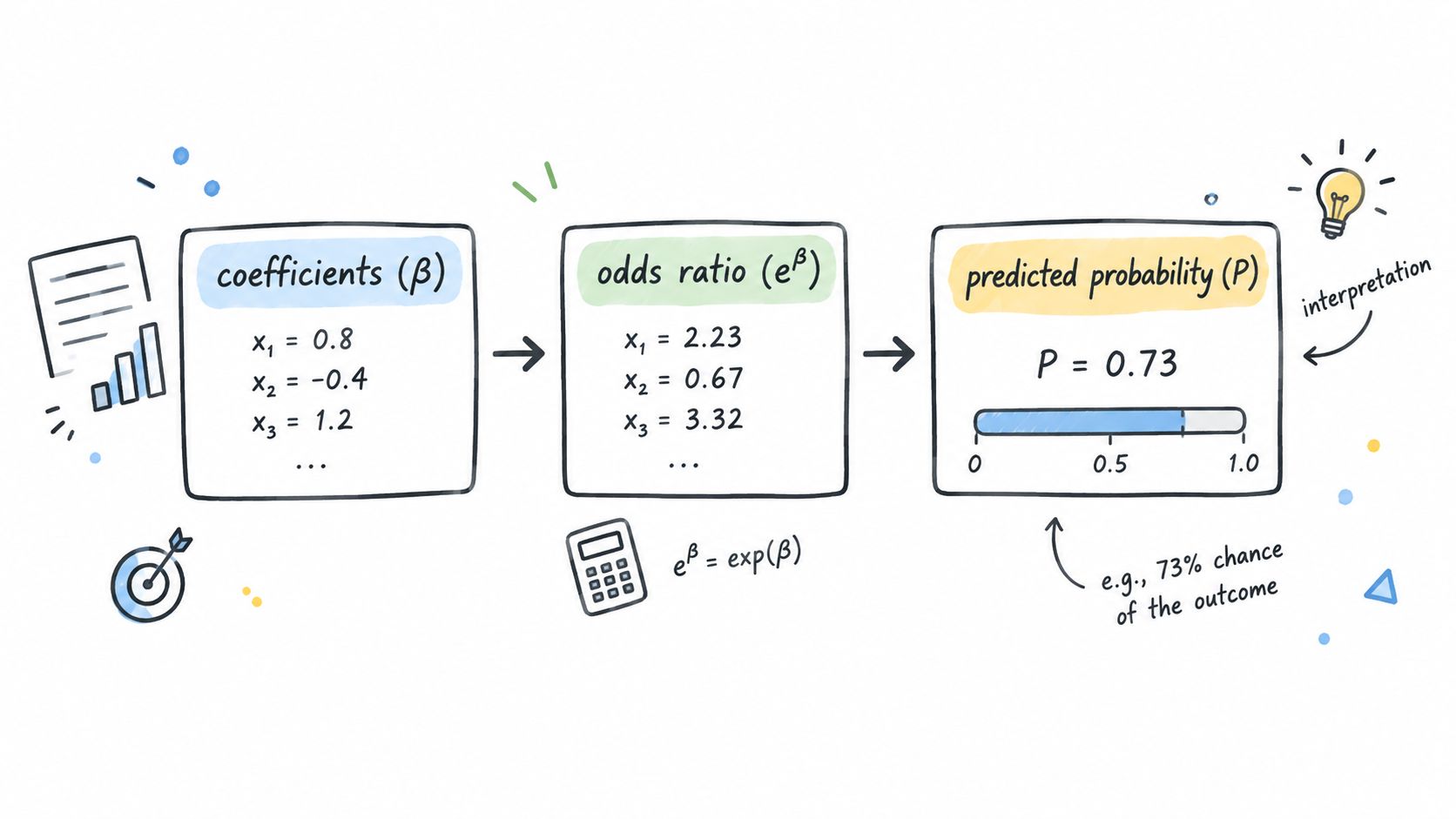
Raw coefficients from a multinomial logit model are just the beginning. The question that actually matters isn't whether a coefficient passes some significance threshold — it's how that coefficient reshapes the probability of each outcome relative to your baseline category.

Turn Coefficients Into Odds Ratios

Let's say car is your reference outcome, and the coefficient for income in the bus equation comes out to -0.04. That number represents the change in log-odds of choosing bus over car for each one-unit bump in income. Exponentiate it and you get the odds ratio:

[
\exp(-0.04) \approx 0.96
]

So each additional unit of income multiplies the bus-versus-car odds by about 0.96, everything else held equal. Notice what this doesn't say — it doesn't mean a 4-percentage-point drop in the probability of choosing bus. The effect operates on relative odds, not absolute probability.

Coefficients shift log-odds. Odds ratios shift relative odds. Neither one is a probability change in disguise.

Good interpretation means anchoring everything to the reference category, being specific about units, reporting confidence intervals, and picking a realistic change in the predictor. Describing what happens when income moves from its 25th to 75th percentile almost always tells a more useful story than a one-unit increment.

Get Probabilities and Marginal Effects

Predicted probabilities are what make model output legible to anyone outside the stats department. For a commuter choosing between car, bus, and train, you'd calculate each probability under a specific set of travel times, costs, and income — then rerun the scenario after, say, a fare increase or a faster bus route.

The workflow looks like this:

1. Pick covariate values that reflect a realistic scenario.
2. Compute the linear predictor for each alternative.
3. Run those through the softmax function to get probabilities.
4. Compare the before-and-after probability profiles.
5. Report both the magnitude of the change and the uncertainty around it.

Marginal effects distill the probability shift associated with a predictor while letting all the alternatives interact. Since probabilities across all options must sum to one, boosting the likelihood of one choice inevitably pulls probability mass from the others — and marginal effects capture that redistribution.

For a deeper walkthrough of how to present this kind of output, see this guide on interpreting regression results.

Ground Your Decisions in More Than Significance

A price coefficient can be razor-significant and still move market share by a fraction of a percent. Conversely, a noisy estimate might be the one that matters most for policy or planning. The right approach is always to pair statistical significance with effect sizes, confidence intervals, predicted probabilities, and real-world context — never let a p-value tell the whole story.

PlotStudio AI can generate narrative interpretations alongside the Python code and computed outputs. That lets you check whether coefficient signs line up with theory, verify model assumptions, and save the entire investigation as a structured Analysis Page rather than a one-off chat response you can't reproduce.

The same probabilities that describe individual choices can also explain market share, ridership, and adoption rates. In marketing, multinomial logit models connect product attributes — price, availability, brand appeal — with the proportion of purchases each option captures.

From Individual Choice to Market Shares

Think of a market as thousands of individual decisions happening simultaneously. Each consumer picks one product. The sales table at the end of the quarter is just the sum of all those picks. A softmax function converts the estimated utilities into shares that sum to one, which makes the model practical even when you don't have access to individual-level choice data. PyMC Labs walks through this aggregated approach in a discrete-choice sales analysis worth reading.

An analyst working with toothpaste sales, for example, might estimate how price and shelf availability shift purchases across brands. Once the model fits, you can simulate a new product launch, a price increase, or pulling a SKU entirely — then compare predicted shares across each scenario.

Market-share analysis turns a choice model into a counterfactual tool. It asks not just what happened, but how the competitive picture might shift if prices, products, or service attributes changed.

Cooper and Nakanishi developed share equations for marketing applications through the 1980s. These equations support market-level decisions rather than predictions for a single respondent, which opened up a whole category of strategic analysis that wasn't possible before.

Practical Business and Policy Uses

Multinomial logit models earn their keep when alternatives compete for the same pool of demand. The most common applications:

• Product launches, estimating whether new sales are incremental or cannibalized from existing products
• Pricing decisions, predicting how a price change redistributes demand across the category
• Transport planning, forecasting ridership after fare changes, route adjustments, or schedule shifts
• Public policy, estimating adoption across competing programs or service options
• Market research, translating stated survey preferences into predicted choice shares

But the basic model has a known weakness: it distributes lost share too evenly. If a new children's product enters a category, it might mostly steal from similar products rather than competing equally with everything else on the shelf. That pattern is a red flag for IIA violation and often justifies moving to a nested or mixed logit specification — MetricGate's comparison of multinomial and conditional logit models covers that decision in useful detail.

Working with Aggregated Data

Aggregated sales data demands careful attention to the denominator. You need total category demand, product availability, observation periods, and consistent definitions of what counts as the market and what counts as a price. Missing products or shifting choice sets can distort predicted shares badly — especially if you treat an unavailable option as genuine zero demand.

PlotStudio AI can inspect uploaded sales or survey data, propose a share-model specification, generate Python code, and preserve the assumptions, charts, predictions, and counterfactual scenarios in an Analysis Page. Its agentic analytics workflow supports ongoing investigation rather than one-shot interpretation. That said, the researcher remains responsible for validating the market definition, causal assumptions, and substitution logic — no tool substitutes for that judgment.

A Practical Share-Model Workflow

1. Define the market and eligible alternatives for each period.
2. Check for missing data, availability shifts, duplicate products, and changing choice sets.
3. Specify utility using prices, attributes, and alternative-specific constants.
4. Estimate observed shares and inspect fit across products and time.
5. Simulate realistic interventions with uncertainty intervals.
6. Compare simple, nested, or mixed specifications when substitution appears uneven.

Done well, you end up with a defensible bridge between micro-level preferences and macro-level outcomes. Just remember to treat counterfactual predictions as model-based scenarios, not guaranteed forecasts.

A fitted model is not automatically a trustworthy model. For multinomial logit models, validation should examine fit, specification, predictors, and whether the results hold up under reasonable changes.

Check Fit and Predictor Quality

Start with a likelihood-ratio test comparing your fitted model against an intercept-only null model. A significant result tells you the predictors improve fit, but it doesn't prove the model is correctly specified. That distinction matters more than people think.

Report a pseudo-R² — McFadden's measure is the standard choice — alongside a few other diagnostics:

• Log-likelihood, for comparing nested specifications
• Classification accuracy, always interpreted against class imbalance
• Confusion matrices, to pinpoint which alternatives the model struggles with
• Predicted probabilities, which often tell you more than hard classifications ever will

Pay attention to standard errors, confidence intervals, and correlations among your predictors. Severe multicollinearity can inflate uncertainty and make coefficient signs flip around, even when the overall fit looks perfectly fine. If removing one variable sharply changes the uncertainty around the others, that's not just a statistical quirk — it's a substantive finding worth reporting.

Good fit is necessary, but it is not evidence that the behavioral story is correct.

Test Assumptions and Robustness

The biggest specification risk remains IIA — the independence of irrelevant alternatives assumption. Omitting a relevant alternative, or treating close substitutes as unrelated, can produce substitution patterns that make no real-world sense. Use Hausman-McFadden comparisons carefully, then check whether dropping alternatives materially changes your coefficients, predicted probabilities, or conclusions.

Watch out for separation and perfect prediction. If one predictor almost perfectly identifies an outcome, maximum-likelihood estimates can blow up — huge coefficients, unreliable standard errors, and a model that looks broken even when the data is telling you something real. Sparse categories, rare choices, and small cells create similar headaches.

Here's a practical checklist worth running through:

1. Re-estimate with alternative-specific constants and see if anything shifts.
2. Compare complete-case results against imputed datasets.
3. Test meaningful subsamples or different time periods.
4. Look for influential observations and unusual predicted probabilities.
5. Compare multinomial, nested, or mixed specifications when substitution patterns look uneven.

Ignoring scale heterogeneity — where different respondents vary in how consistently they make choices — can quietly bias comparisons across groups. And when you have repeated choices from the same person, the independent-observation assumption deserves serious scrutiny.

For handling uncertainty under clustering or heteroskedasticity, learn more about robust standard errors.

Use AI Without Delegating Judgment

PlotStudio AI can run a multi-step diagnostic workflow, surface potential issues, execute Python locally, and preserve code, tests, charts, and explanations in an Analysis Page. This is agentic analytics, not just a generated paragraph of interpretation.

But here's the catch. A flagged IIA concern might reflect a genuine model failure — or it might be a defensible simplification given your study design. Only the researcher can decide which interpretation fits.

Finally, save the full analysis pipeline — data preparation, model formula, reference category, software versions, diagnostics, and sensitivity analyses. Reproducibility depends on documenting how you got the result, not just the final table you're putting in the report.

When Should Researchers Use MNL?

Reach for multinomial logit models when your alternatives have no natural ordering, the IIA assumption is defensible in your context, and you need something straightforward to estimate. That said, if your choices cluster into obvious substitutes, nested logit usually fits better. When you need to account for correlation between alternatives, multinomial probit gives you that flexibility — at the cost of more demanding estimation.

How Many Observations Do You Actually Need?

There's no magic number. The old 10–20 observations per parameter rule is a starting point, not gospel. What matters more is how your outcome categories are distributed, whether you're running into separation issues, how much data is missing, and how the model performs on validation. When sample size is tight, penalized estimation or a leaner specification can keep things stable.

Can MNL Handle Repeated Choices?

Not in its basic form — standard MNL treats each observation as independent. When you're working with panel data or the same respondents making multiple choices, you'll want a mixed logit extension that incorporates respondent-level random effects or coefficients. Don't forget to cluster your standard errors, either.

How Should Results Be Reported?

Always state your reference category upfront. Report coefficients, odds ratios, confidence intervals, diagnostics, and the full model specification. But here's where the real clarity comes in: predicted probabilities and marginal effects tell the story that raw log-odds simply can't. Stakeholders understand "a 12-point increase in probability" far better than they understand log-odds coefficients.

PlotStudio AI can document each of these steps in reproducible Analysis Pages, while keeping methodological decisions firmly in the researcher's hands. Researchers can try PlotStudio AI with discounted academic pricing and 1,000 free credits.