Multiple Testing Correction: A Practical Guide for Researchers

Multiple testing correction adjusts significance thresholds or p-values when you run more than one hypothesis test on the same dataset, so your reported error rate reflects the whole set of tests instead of just one. The short rule of thumb: use familywise error rate (FWER) control, such as Holm or Bonferroni, for a small number of pre-specified confirmatory comparisons, and use false discovery rate (FDR) control, such as Benjamini-Hochberg, for large exploratory screens where you expect many true effects and can tolerate a controlled fraction of false leads.
Here is why this matters more than most researchers assume. Run 10,000 independent tests on true null hypotheses at α = 0.05, and you will get roughly 500 false positives by chance alone, not because anything went wrong with your data, but because that is what a 5% error rate does at scale. A single genomics screen or a battery of psychology subscale comparisons can easily reach that order of magnitude. If you do not correct for it, your “discoveries” section is mostly noise dressed up as signal.
Pro Tip: Before you touch a p-value, decide whether you are confirming a hypothesis you specified in advance or exploring a dataset for candidates worth following up. That single decision determines whether you reach for Holm or for Benjamini-Hochberg, and it should happen before you look at results, not after.
Key Takeaways
Choosing between FWER and FDR control, matching the method to whether your analysis is confirmatory or exploratory, and pre-specifying the correction before seeing results are what separate defensible multiple testing correction from statistical theater.
| Point | Details |
|---|---|
| Match error rate to intent | Use FWER (Holm) for small confirmatory tests, FDR (BH or Storey) for large exploratory screens. |
| Ten thousand tests, 500 false positives | Uncorrected testing at α = 0.05 across 10,000 true nulls yields roughly 500 false positives on average. |
| Holm beats plain Bonferroni | Holm’s step-down procedure controls FWER with uniformly greater power than Bonferroni. |
| Dependence changes the guarantee | BH needs independence or PRDS; use Benjamini-Yekutieli or permutation methods under arbitrary dependence. |
| Define the family before you look | Pre-specify which tests count as one family before seeing results to avoid post-hoc correction bias. |
| Reproducible correction pipelines | Plotstudio runs Holm, BH, BY, and Storey’s q-value natively in R and Python with an audit trail for each analysis plan. |
Table of Contents
- What Is Multiple Testing Correction and Why Do You Need It?
- FWER vs FDR: How Do You Choose the Right Error Rate?
- What Are the Main Multiple Comparisons Correction Methods?
- Why Do These Procedures Actually Control Their Target Error Rate?
- When Should You Apply a Multiple Testing Correction?
- How Do You Implement Corrections in R and Python?
- A Step-By-Step Worked Example of Bonferroni and BH Corrections
- What Mistakes Do Researchers Make With Multiple Comparisons Correction?
- How Does Multiple Testing Correction Change at Genomic Scale?
- Key Multiple Testing Correction Takeaways for Your Next Analysis
- Where Can You Learn More About Multiple Comparisons Correction?
- An Editorial Take on Getting Multiplicity Right
- How PlotStudio Supports Reproducible Multiple Testing Workflows
- Frequently Asked Questions About Multiple Testing Correction
- Sources
What Is Multiple Testing Correction and Why Do You Need It?
Multiple hypothesis testing means running more than one statistical test against the same dataset, whether that is 20 gene comparisons, 15 subgroup analyses, or a single primary endpoint checked at three time points. Each individual test carries its own false positive risk, typically capped at α = 0.05. Run several of them, and those risks compound.
The intuition is simple: if any single coin flip has a 5% chance of landing on a result you would call “significant” by pure chance, then flipping that coin 20 times raises the odds that at least one flip comes up “significant” well above 5%. Statisticians formalize this with the familywise error expression:
α̅ = 1 − (1 − α)^m
where α is your per-test significance level and m is the number of tests. With m = 20 tests at α = 0.05, the probability of at least one false positive climbs to roughly 64%, not 5%. For situations where tests are not independent, Boole’s inequality gives a simpler conservative bound: α̅ ≤ m × α, which holds regardless of dependence structure and is the basis for the Bonferroni correction.
The numbers get dramatic at scale. Testing 10,000 independent true null hypotheses at α = 0.05 produces about 500 false positives on average, even though none of the underlying effects are real. That is the exact scenario a genome-wide association study or a differential expression analysis runs into routinely, which is why almost no serious genomics paper reports raw, uncorrected p-values.
A few things worth internalizing before you pick a method:
- The inflation is a property of the number of tests, not of your data quality or study design.
- It applies whether the tests are formally “hypotheses” in a paper or informal comparisons you run while exploring a dataset.
- Correction does not fix a flawed experiment; it only keeps your error accounting honest for the number of comparisons you actually ran.
- The size of the problem scales roughly linearly with m under the Bonferroni bound, which is exactly why blanket correction becomes unworkable at genomic scale.
FWER vs FDR: How Do You Choose the Right Error Rate?
Familywise error rate and false discovery rate answer different questions, and conflating them is one of the more common errors in applied statistics. FWER asks: what is the probability of making even one false discovery across the entire family of tests? Formally, FWER = P(V ≥ 1), where V counts the number of true nulls incorrectly rejected. FDR asks a different question: among all the discoveries you report, what fraction do you expect to be false? Formally, FDR = E[V/R], the expected proportion of false positives among rejections R, with the ratio conventionally set to zero when R = 0.
That distinction changes what each method is good for. FWER control is strict: it protects against ever declaring a false positive across the whole set, which is why it dominates confirmatory research, clinical trials, and any setting where a single wrong claim carries real consequences. FDR control is more permissive by design: it accepts that some fraction of your reported hits will be false, in exchange for detecting far more true effects when you are running hundreds or thousands of tests.
Familywise error rate and false discovery rate are not two flavors of the same correction. FWER guards the probability of any false positive across every test; FDR budgets the expected proportion of false positives among the discoveries you actually report. Picking the wrong one for your research question either wastes power or overstates your findings.
When each one fits:
- Target FWER when you have a small number of pre-registered, confirmatory comparisons, such as testing a primary endpoint plus two secondary endpoints in a clinical trial, or comparing three treatment arms against a control.
- Target FWER in regulatory contexts, where a single false claim has legal or safety consequences and reviewers expect strict family-wide control.
- Target FDR when you are screening large numbers of candidates, such as thousands of genes, SNPs, or voxels, and you plan to follow promising hits with independent validation anyway.
- Target FDR when statistical power matters more than airtight certainty on any single result, because FWER methods lose power fast as the number of tests grows.
- One Journal of Clinical Epidemiology letter makes a point worth remembering: FDR is not a universal upgrade over Bonferroni. It is a different tool for a different inferential goal, and using it where FWER control is expected can understate how uncertain your results really are.
What Are the Main Multiple Comparisons Correction Methods?
Several correction procedures exist, and they differ in what error rate they control, how conservative they are, and what assumptions about test dependence they require. Here is how the major methods stack up.
| Method | Error Rate Target | Conservativeness / Power | Assumptions | Best For | Implementation |
|---|---|---|---|---|---|
| Bonferroni | FWER | Most conservative, lowest power | Works under any dependence | Small n, strict confirmatory tests | Trivial: multiply p by m |
| Holm (Holm-Bonferroni) | FWER | Uniformly more powerful than Bonferroni | Any dependence | Confirmatory tests, default FWER choice | Step-down, easy in most software |
| Šidák | FWER | Slightly more powerful than Bonferroni | Assumes independence | Independent small-n tests | Simple closed-form formula |
| Hochberg | FWER | More powerful than Holm in some cases | Requires non-negative dependence | Moderate n, mild dependence | Step-up procedure |
| Benjamini-Hochberg (BH) | FDR | Considerably more powerful at large m | Independence or positive dependence (PRDS) | Exploratory large-scale screens | Step-up, widely implemented |
| Benjamini-Yekutieli (BY) | FDR | More conservative than BH | Arbitrary dependence | Correlated tests with unknown structure | Same step-up logic, harsher penalty |
| Storey’s q-value | FDR | Often more powerful than BH | Independence or PRDS; estimates π₀ | Genomics, large screens with many true effects | Requires π₀ estimation software (qvalue package) |
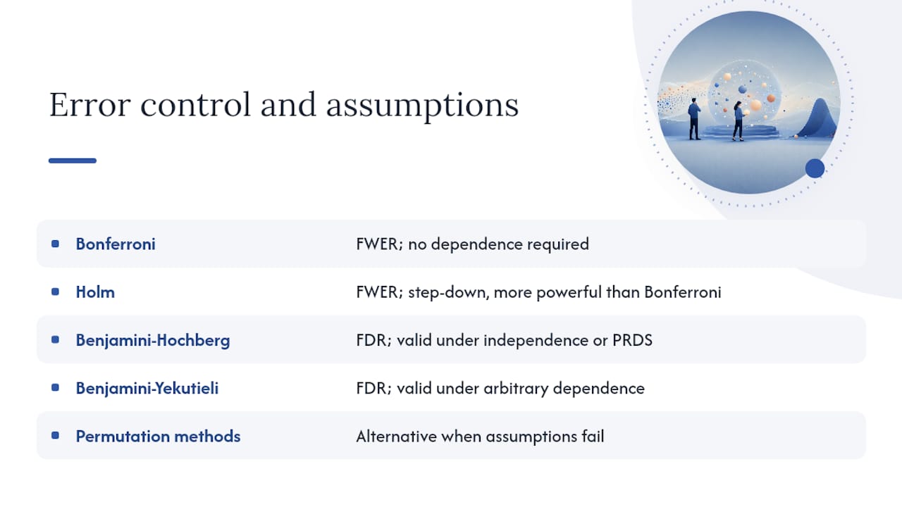
Bonferroni is the simplest and most conservative method: multiply each p-value by the number of tests, or equivalently divide α by m. It works under any dependence structure between tests, which is its main virtue, but it sacrifices power aggressively as m grows.
Holm’s step-down procedure fixes much of that weakness. It sorts p-values from smallest to largest and compares each one to a progressively looser threshold, which means it uniformly outperforms Bonferroni in power while still guaranteeing the same FWER control. There is rarely a good reason to run plain Bonferroni when Holm is available in the same software function and costs nothing extra.
Benjamini-Hochberg is the workhorse of FDR control. It also sorts p-values and applies a step-up threshold that scales with rank, and it controls FDR under independence and under certain positive dependence structures known as PRDS. When test dependence is arbitrary or unknown, Benjamini-Yekutieli applies a more conservative correction factor that guarantees FDR control regardless of correlation structure, at the cost of reduced power.
Storey’s q-value approach improves on BH by estimating π₀, the proportion of hypotheses that are truly null, rather than assuming it is 1. In real screens, particularly genomic ones, a meaningful fraction of tested hypotheses are genuinely non-null, and accounting for that can recover real power without inflating the false discovery rate.
For picking a method in practice: confirmatory small-n work almost always calls for Holm. Exploratory large-n screens almost always call for BH or Storey’s q-value. When tests are known to be strongly and arbitrarily correlated, and you cannot assume PRDS, BY is the safer default even though it costs power.
Why Do These Procedures Actually Control Their Target Error Rate?
You do not need to take these guarantees on faith. The proofs are short enough to sketch and worth understanding, because they tell you exactly where each method’s guarantee breaks down.
Bonferroni’s FWER control follows directly from Boole’s inequality. If you reject any of m null hypotheses at threshold α/m, the probability that at least one true null is falsely rejected is at most the sum of the individual rejection probabilities, each bounded by α/m. Summed across m tests, that union bound gives P(at least one false rejection) ≤ m × (α/m) = α. This holds no matter how the tests are correlated, which is exactly why Bonferroni remains valid even when you know nothing about test dependence.
Holm’s step-down procedure achieves the same FWER bound with a cleverer argument. Instead of testing every hypothesis against α/m, it tests the smallest p-value against α/m, the next smallest against α/(m−1), and so on. The step-down structure preserves the same union-bound logic at each stage while relaxing the threshold for later comparisons, which is why it dominates Bonferroni in power without giving up any FWER guarantee.
Benjamini-Hochberg’s FDR argument is different in character. Under independence, the expected proportion of false discoveries among rejections can be shown to equal exactly α × (m₀/m), where m₀ is the number of true nulls, which is bounded above by α. The proof relies on the ordering of p-values and a martingale-style argument across the sorted sequence. Under positive regression dependence (PRDS), the same bound still holds, which is why BH remains valid for many correlated-test scenarios common in genomics. Under arbitrary negative dependence, the guarantee can fail, which is precisely the gap that Benjamini-Yekutieli’s more conservative multiplier closes.
The guarantee behind every correction method rests on a specific dependence assumption. Bonferroni and Holm need none. Benjamini-Hochberg needs independence or PRDS. Step outside those assumptions without switching to BY or a permutation-based method, and your stated error rate stops being true, even though the arithmetic still runs.
Pro Tip: If you are not sure whether your tests satisfy PRDS, a quick empirical check is to look at the sign of pairwise correlations between test statistics. Predominantly positive correlations are a reasonable, though not airtight, signal that BH’s assumptions are roughly satisfied.
When Should You Apply a Multiple Testing Correction?
Deciding whether and how to correct is a design decision, not an afterthought you bolt on after seeing results. Work through this checklist before you run a single test:
- Define the family of tests explicitly. Decide up front which comparisons belong together as one family, whether that is every gene in an experiment or every subgroup comparison in a trial. The family definition determines your m, and changing it after seeing results is a form of p-hacking.
- Classify the analysis as confirmatory or exploratory. A pre-registered primary hypothesis calls for FWER control. A hypothesis-generating screen calls for FDR control. Mixed studies should separate confirmatory and exploratory tests into distinct families with different correction targets.
- Pre-register the correction method and threshold. State your chosen method, your target α or q-value, and the number of planned tests before collecting or analyzing data. This closes off the temptation to try several methods and report whichever produces the cleanest result.
- Run power calculations that account for multiplicity. A sample size calculated for a single test at α = 0.05 will be underpowered once you divide that threshold across 20 comparisons. Build the correction into your power analysis, not just your final significance test.
- Avoid post-hoc family redefinition. Do not decide, after seeing which tests look promising, that only those tests count as “the family” for correction purposes. That maneuver defeats the entire purpose of correcting in the first place.
- Report the full methodology in your write-up. State which correction method you used, why you chose it, how many tests were in the family, and whether you are reporting adjusted p-values, adjusted α thresholds, or both.
How Do You Implement Corrections in R and Python?
Implementation is where good intentions meet software defaults, and the defaults matter more than most researchers realize.
In R, the base function is p.adjust(p, method, n), which supports holm, hochberg, hommel, bonferroni, BH, BY, and fdr as method arguments, with fdr as an alias for BH. The n argument specifies the number of comparisons and defaults to the length of the input vector, which creates a subtle trap: if you only pass in the p-values you consider “interesting” rather than the full set of tests you ran, p.adjust will correct for the wrong m and understate the true multiplicity.
DESeq2, the standard tool for RNA-seq differential expression analysis, applies Benjamini-Hochberg correction by default to every gene tested, reporting the result in its padj column. That default reflects the field’s general acceptance that FDR, not FWER, is the appropriate error rate for genome-wide screens involving tens of thousands of genes. Researchers who report DESeq2’s raw p-values instead of padj are, whether they realize it or not, ignoring the correction the tool already applied and is designed around.
In Python, statsmodels.stats.multitest.multipletests provides equivalent functionality, accepting a method argument (bonferroni, holm, fdr_bh, fdr_by, and others) and returning both a boolean rejection array and the array of adjusted p-values. A common implementation mistake is applying corrections separately to subsets of tests analyzed in different scripts or notebooks, which silently changes m and breaks the guarantee the method is supposed to provide.
Whatever software you use, the correction is only as honest as the m you feed it. Filtering your p-value list to “the ones that look interesting” before calling p.adjust or multipletests is not a shortcut. It is a different, uncorrected analysis wearing a corrected analysis’s clothing.
A few practical notes worth keeping in mind: adjusted p-values and adjusted α thresholds are mathematically equivalent ways of expressing the same decision, so pick whichever your field’s reporting conventions expect. Missing p-values (NA in R, NaN in Python) should be excluded from the correction rather than silently included as zeros or dropped after the fact, since either mishandling changes your effective m. And if some planned tests were never run because of missing data or failed assays, m should reflect the tests you actually observed, not the tests you originally planned.
A Step-By-Step Worked Example of Bonferroni and BH Corrections
Nothing clarifies the difference between FWER and FDR control faster than running both on the same ten p-values and watching what changes. Suppose an experiment produces the following raw p-values, ranked from smallest to largest.
Bonferroni’s adjustment is arithmetic: multiply each raw p-value by m = 10 (capped at 1.0). Only the smallest raw p-value, 0.001, survives at the 0.05 threshold after that multiplication, since its adjusted value of 0.010 is the only one under 0.05.
BH works differently. Rank the p-values from smallest to largest, then compare each one to (rank/m) × α, working from the largest rank downward and carrying forward the smallest qualifying threshold to preserve monotonicity. Here, five tests clear the BH threshold rather than one.
Interpretation matters as much as the arithmetic. Declaring significance under Bonferroni means you are controlling the probability of even one false positive across all ten tests at 5%, a strict guarantee. Declaring the five BH-flagged results as discoveries means you expect roughly 5% of those five discoveries, about a quarter of one result, to be false positives, a different and more permissive kind of guarantee. Neither number is “more correct” in the abstract. They answer different questions.
- Rank raw p-values from smallest to largest and record the rank i for each.
- For Bonferroni, multiply each raw p-value by m (the total number of tests), capping at 1.0.
- For BH, compute (i/m) × α for each rank i, then find the largest rank where the raw p-value is below that threshold, and declare that rank and all smaller ranks significant.
- Report both the method used and the number of tests in the family alongside the adjusted values.
In R, this is one line: p.adjust(p_values, method = "BH") or method = "bonferroni". In Python, statsmodels.stats.multitest.multipletests(p_values, method='fdr_bh') returns the same result along with a boolean significance mask.
What Mistakes Do Researchers Make With Multiple Comparisons Correction?
The most damaging mistake in applied multiple hypothesis testing is defining the family of tests after seeing the results. Running 50 comparisons, noticing that five look promising, and then correcting only those five as if they were the entire family defeats the purpose of correction entirely. The family has to be fixed before you see outcomes, or the correction is theater.
A second common error is applying Bonferroni reflexively to massive screens where it is simply the wrong tool. At m = 20,000, Bonferroni’s threshold of 0.05/20,000 = 0.0000025 is so strict that almost nothing survives, even genuinely real effects. At that scale, near-zero power is the predictable outcome of using an FWER method built for confirmatory, not exploratory, purposes.
A third mistake is ignoring test dependence structure entirely. Applying BH without checking whether PRDS holds, when your tests are strongly and arbitrarily correlated, can understate your true false discovery rate. Switching to BY or a permutation-based approach closes that gap at the cost of some power.
A fourth, subtler error is treating FDR as a per-test probability rather than a rate across the batch of discoveries. An individual result with a BH-adjusted q-value of 0.03 is not “3% likely to be a false positive” in isolation.
Correction is not a box to check after you have already decided which results matter. The moment you select “promising” tests before applying a correction, you have already broken the guarantee the correction was supposed to provide, no matter how carefully you compute the adjusted p-values afterward.
Avoiding these mistakes comes down to discipline established before analysis: pre-specify the family, choose the error rate that matches your actual research goal, and treat any striking discovery from a large screen as a hypothesis for independent replication rather than a finished result.
How Does Multiple Testing Correction Change at Genomic Scale?
Genomics, neuroimaging, and other high-throughput fields push multiple testing correction into territory where the standard confirmatory playbook simply does not work. Testing tens of thousands of genes or hundreds of thousands of voxels means Bonferroni’s threshold becomes so conservative that true effects routinely fail to clear it, regardless of effect size. This is the core reason FDR control, not FWER control, is the default expectation in these fields.

Dependence between tests is the second major complication at scale. Genes in the same pathway, or voxels in the same brain region, are correlated by biology, not by chance. When that dependence is positive and PRDS-compatible, standard BH remains valid. When it is not, researchers turn to permutation-based methods that estimate the null distribution empirically from the data itself, sidestepping the need to assume a particular dependence structure altogether.
Storey’s approach to estimating π₀, the proportion of hypotheses that are truly null, adds real power in fields where a meaningful fraction of tests represent genuine effects. Rather than assuming every null hypothesis is true, as basic BH implicitly does when computing its threshold, Storey’s method estimates π₀ directly from the p-value distribution and adjusts the FDR calculation accordingly. Related tools include empirical null modeling, which estimates the actual null distribution of test statistics from the bulk of the data rather than relying on theoretical assumptions, and local FDR, which estimates a false discovery probability for each individual test rather than a batch-wide rate.
- Permutation-based FWER and FDR control estimate significance thresholds directly from resampled data, avoiding reliance on distributional assumptions that may not hold at scale.
- Independent cohort replication remains the gold standard for validating high-throughput findings, regardless of which correction method flagged them.
- Reporting the expected number or proportion of false discoveries alongside your correction method gives readers a concrete sense of how much noise to expect in your reported hit list.
Pro Tip: When a high-throughput screen returns far more “significant” hits than you expected, check your π₀ estimate before assuming you found something extraordinary. A poorly estimated π₀ close to 1 when the true value is much lower will understate your effective power and can mislead you about how conservative your results really are.
Key Multiple Testing Correction Takeaways for Your Next Analysis
Choosing the right multiple testing correction means matching the error rate to your research intent, defining the test family before you see results, and reporting the exact method and adjusted values you used.
- Define the family of tests before running any analysis, not after seeing which results look interesting.
- Use FWER control (Holm over plain Bonferroni) for small, pre-specified confirmatory comparisons.
- Use FDR control (Benjamini-Hochberg or Storey’s q-value) for large exploratory screens where power matters more than airtight per-test certainty.
- Report the correction method, the number of tests in the family, and either adjusted p-values or adjusted α thresholds in your methods section.
- Treat striking discoveries from large screens as candidates for independent replication, not as finished conclusions.
Where Can You Learn More About Multiple Comparisons Correction?
A short list of primary sources will take you further than most secondhand summaries, including this one.
- Benjamini and Hochberg’s 1995 paper established the step-up FDR procedure and remains the definitive reference for understanding why and how it controls the false discovery rate under independence and PRDS dependence.
- Holm’s 1979 paper introduced the step-down FWER procedure that improves on Bonferroni’s power while preserving its guarantee, and it remains the standard citation for justifying Holm as a default FWER method.
- The Wikipedia overview of the multiple comparisons problem is a useful quick reference for formal definitions, correction formulas, and a concise summary of when to prefer FWER versus FDR.
- Noble’s 2009 explainer on multiple testing correction walks through why high-throughput biology needed a departure from classical FWER methods and how FDR and permutation approaches filled that gap.
- The R documentation for p.adjust is the fastest way to confirm exact method names, default arguments, and the n-argument caveat before running an analysis.
- The J Clin Epidemiology letter on FDR versus Bonferroni is worth reading in full for its argument that the two error rates serve different inferential goals and should not be swapped interchangeably.
An Editorial Take on Getting Multiplicity Right
Most disputes over multiple testing correction are not actually disputes about statistics. They are disputes about what a paper is claiming to have found. A researcher who runs 40 subgroup comparisons and reports the three that survived uncorrected wants those three findings to be confirmatory conclusions, but the analysis behind them was exploratory the entire time. Correction does not resolve that mismatch. It exposes it.
The pragmatic middle ground I keep coming back to is this: power and error control are genuinely in tension, and no correction method escapes that tradeoff, it only moves where you sit on it. Holm buys you a strict guarantee at the cost of missing real effects in anything beyond a handful of tests. Benjamini-Hochberg buys you power at the cost of accepting that a defined fraction of your reported hits are wrong. Neither choice is more rigorous than the other in the abstract. The rigor comes from choosing deliberately, before you see your data, and being honest in your methods section about which choice you made and why.
Pre-registration and reproducible audit trails are the closest thing this field has to an antidote for the abuse that gives correction methods a bad name. A pre-specified analysis plan that states the family, the method, and the threshold before data collection removes the temptation to shop for whichever correction produces the cleanest table. That discipline matters more than which specific method you pick.
How PlotStudio Supports Reproducible Multiple Testing Workflows
Getting the correction right is one problem. Proving to a reviewer, supervisor, or co-author exactly which method you used, on exactly which set of tests, and why, is a separate and often harder one. Plotstudio closes that gap by making the multiplicity decision part of an analysis plan you approve before any code runs, rather than a choice buried in a script nobody else can trace.

Plotstudio runs both R and Python natively and supports Holm, Benjamini-Hochberg, Benjamini-Yekutieli, and Storey’s q-value out of the box, so switching between FWER and FDR control for a confirmatory versus exploratory analysis takes a plan revision, not a rewrite. Every run produces an audit trail documenting the exact method, the family size, and the adjusted values reported, which is the kind of documentation a thesis committee or peer reviewer will ask for eventually anyway. Because analysis runs locally on your own machine, this works even for IRB-governed or patient-level datasets that cannot leave the device for a cloud tool. If you are choosing between correction methods for an upcoming submission, you can see how Plotstudio’s agentic analytics platform handles the full workflow, from raw p-values to a reproducible report, and start a trial to run your own dataset through it.
Frequently Asked Questions About Multiple Testing Correction
What is multiple testing correction in simple terms? It is a set of statistical adjustments applied when you run more than one hypothesis test on the same data, designed to keep your overall false positive rate honest instead of letting it inflate with every additional test.
Should I use Bonferroni or Benjamini-Hochberg? Use Bonferroni-family methods (Bonferroni or, better, Holm) for a small number of pre-specified confirmatory tests where any single false positive is costly. Use Benjamini-Hochberg for larger exploratory screens where you want to maximize true discoveries and can tolerate a controlled false discovery proportion among your reported hits.
Does DESeq2 apply multiple testing correction automatically?
Yes. DESeq2 applies Benjamini-Hochberg correction by default and reports the result in its padj column, reflecting the standard practice of using FDR control for genome-wide differential expression testing.
What is the difference between an adjusted p-value and a q-value? An adjusted p-value from Bonferroni or Holm tells you the threshold at which a single test would remain significant under FWER control. A q-value from Benjamini-Hochberg or Storey’s method tells you the minimum FDR at which that test would be called significant, which is a statement about expected false discoveries across a batch, not about that test alone.
Do I always need to correct for multiple comparisons? Not always. Correction is strictly justified when you are drawing a single conclusion from a collective omnibus null tested piecewise, or when the family of tests genuinely represents one research question. Applying correction reflexively to every comparison in a paper, regardless of whether they form a meaningful family, can be as misleading as not correcting at all.
Can I use FDR control instead of Bonferroni for a clinical trial? Generally no, for primary and secondary confirmatory endpoints. Regulatory and confirmatory settings typically expect FWER control because a single false claim carries real consequences. FDR control fits exploratory analyses within the same trial, but the primary confirmatory endpoints usually still call for FWER methods like Holm.
Sources
- A general introduction to adjustment for multiple comparisons
- R: Adjust P-values for Multiple Comparisons
- Multiple testing lecture notes (UCDavis teaching files)
- Multiple comparisons problem — Wikipedia
- False discovery rate control is not always a replacement for Bonferroni adjustment (Letter commenting on: J Clin Epidemiol. 2014;67:850-7)