Propensity Score Matching: A Practical Guide for Researchers

Propensity score matching (PSM) estimates the average treatment effect on the treated by pairing each treated unit with one or more control units that share a nearly identical probability of receiving treatment given observed covariates. Use it when your estimand is the ATT, when you have enough controls to find good matches, and when you can defend conditional exchangeability and sufficient overlap in your data. The canonical workflow runs in five steps: estimate the propensity score, check overlap, choose and apply your matching or weighting method, diagnose covariate balance, then estimate the treatment effect with appropriate standard errors and sensitivity analyses.
Before you open R or Python, settle three immediate decisions:
- 1:1 vs. 1:n matching: 1:1 is conservative and clean; 1:n gains precision but with diminishing returns past a ratio of about 3:1.
- Caliper width: the standard guidance is 0.2 standard deviations of the logit of the propensity score; tighter calipers reduce bias but cost you matched sample size.
- Replacement: matching with replacement reduces bias when controls are scarce but requires variance estimation that accounts for repeated use of the same control unit.
Key Takeaways
Propensity score matching estimates the ATT by pairing treated and control units on a single balancing score, but its validity depends entirely on three untestable assumptions, rigorous balance diagnostics, and transparent sensitivity analyses.
| Point | Details |
|---|---|
| Choose estimand before method | Decide ATE vs. ATT before modeling; matching targets ATT, IPTW targets ATE. |
| Caliper at 0.2 SD of logit PS | Austin’s simulation guidance: set caliper at 0.2 SD of the logit of the propensity score to balance bias and sample retention. |
| SMD below 0.1 is the balance threshold | Report standardized mean differences for every covariate pre- and post-matching; the standard threshold is |
| Always run sensitivity analysis | Report the E-value or Rosenbaum bounds; no PSM result is credible without quantifying robustness to unmeasured confounding. |
| Plotstudio for reproducible PSM | Plotstudio runs MatchIt/WeightIt/cobalt workflows locally, gates execution behind a pre-registered plan, and exports full reproducibility packages. |
Table of Contents
- What are the causal assumptions behind propensity score methods?
- How do you estimate a propensity score and avoid common modeling mistakes?
- Which PS method fits your study: matching, weighting, stratification, or covariate adjustment?
- How does propensity score matching work in practice?
- How do you check whether matching achieved covariate balance?
- How do you estimate treatment effects and compute valid standard errors after matching?
- How robust is your PSM result to unmeasured confounding?
- A reproducible five-step checklist for your PSM analysis
- Which R and Python packages should you use for PSM?
- Why reproducibility and privacy matter for PS analyses in regulated research
- The case for choosing your estimand before your method
- Plotstudio runs your PSM workflow locally, with a full audit trail
- Sources
What are the causal assumptions behind propensity score methods?
Rosenbaum and Rubin’s 1983 paper introduced the propensity score as Pr(treatment | observed covariates) and proved it is a balancing score: conditioning on it is sufficient to remove confounding from all observed covariates simultaneously. That result sits inside the potential-outcomes framework, so understanding that framework is the prerequisite for using PSM defensibly.
Potential outcomes and estimands
Each unit i has two potential outcomes: Y(1) under treatment and Y(0) under control. The individual treatment effect Y(1) − Y(0) is never observed for the same unit at the same time. The estimand you choose determines which average you are trying to recover.
- ATE (average treatment effect): E[Y(1) − Y(0)] averaged over the full population. Weighting methods, particularly inverse-probability-of-treatment weighting (IPTW), target this.
- ATT (average treatment effect on the treated): E[Y(1) − Y(0) | T = 1] averaged only over treated units. Matching methods naturally target the ATT because you are constructing a control group that looks like the treated group.
Researchers in clinical and social sciences most often want the ATT: the question is not “what would happen if everyone were treated?” but “did treatment help the people who actually received it?” Matching is the right tool for that question. If your question is population-wide, lean toward weighting.
The three core assumptions
Conditional exchangeability (also called no unmeasured confounding or strong ignorability): given the observed covariates X, treatment assignment is independent of potential outcomes — Y(0), Y(1) ⊥ T | X. Positivity (overlap): every unit has a nonzero probability of receiving either treatment — 0 < Pr(T = 1 | X) < 1 for all X in the support. Consistency: the observed outcome for a treated unit equals its potential outcome under treatment — Y = Y(1) if T = 1.
These three assumptions are described in detail by Austin and colleagues as the foundation for any propensity-score analysis. Conditional exchangeability is the one you cannot verify from data alone; it requires subject-matter judgment about which confounders you have measured. Positivity is checkable: inspect the PS distribution for regions where one group has no support. Consistency is violated when the treatment is not well-defined or when multiple versions of treatment exist.
Practical implication for study design: collect all variables that predict both treatment assignment and the outcome. A variable that predicts only treatment assignment adds noise to the PS model without reducing confounding bias; a variable that predicts only the outcome is better used as a covariate in the outcome model.
How do you estimate a propensity score and avoid common modeling mistakes?
The propensity score is formally defined as e(X) = Pr(T = 1 | X = x). Its value as a balancing score follows directly from the potential-outcomes framework: if you condition on e(X), the distribution of X is the same in treated and control groups in expectation. That property is what makes matching on a single scalar feasible rather than matching on the full covariate vector.
Modeling choices
Logistic regression remains the baseline. It is transparent, easy to report, and well-understood by reviewers. For binary treatment with a moderate number of covariates and no severe nonlinearity, it performs well. For multi-arm studies, multinomial logistic regression extends naturally, and generalized propensity scores for multi-group comparisons are increasingly used when pairwise matching across three or more arms becomes unwieldy.
Machine learning methods, including gradient-boosted trees (as implemented in the twang package) and random forests, can capture nonlinear relationships and interactions that logistic regression misses. The tradeoff is interpretability: a reviewer cannot easily audit a 500-tree forest the way they can audit a logistic regression table. Use ML-based PS estimation when you have strong prior reason to expect nonlinearity and when you report the approach transparently. The twang package in R was designed specifically for this use case, using gradient boosting to optimize covariate balance rather than predictive accuracy.
Variable selection principles
- Include all variables that are causally prior to treatment and plausibly related to the outcome (confounders). This is the set that matters for bias reduction.
- Do not include post-treatment variables. Conditioning on a mediator or a collider opens a backdoor path and can introduce bias rather than remove it.
- Proxy variables for unmeasured confounders can help, but their inclusion requires careful justification.
- High-dimensional covariate spaces (e.g., claims data with hundreds of diagnosis codes) benefit from regularized methods or data-adaptive variable selection, but always check that the selected variables make clinical or theoretical sense.
Pro Tip: Before fitting the PS model, run a data profiling pass on your covariates: check distributions, flag missingness patterns, and identify near-zero-variance variables. A covariate with 95% missing data or zero variance cannot balance anything and will only inflate model uncertainty.
PS model diagnostics
Inspect the PS distribution separately for treated and control units before matching. Overlap plots (mirrored histograms or density plots of the logit of the PS) reveal immediately whether common support exists. If the PS distributions barely overlap, matching will either discard most of your sample or produce poor-quality matches regardless of algorithm.
Common pitfalls to avoid:
- Model misspecification: omitting a strong confounder biases the PS and leaves residual confounding after matching. Sensitivity analyses (Section 8) are your only recourse.
- Including irrelevant covariates: adding noise variables inflates PS variance and can worsen balance on the covariates that matter.
- Failing to report PS model details: reviewers need the full covariate list, model type, and software used to assess your analysis. Omitting these is a reproducibility failure.
Which PS method fits your study: matching, weighting, stratification, or covariate adjustment?
The four main applications of the propensity score differ in their target estimand, how they handle poor overlap, and how much sample they retain. Choosing the wrong one for your question is a common error that no amount of careful diagnostics can fix after the fact.
Matching constructs a pseudo-experimental dataset by pairing treated units with similar controls. It naturally targets the ATT and is intuitive to report. The cost is sample loss: unmatched units are discarded, which reduces precision and can introduce selection if the matched sample is not representative of the treated group.
IPTW (inverse-probability-of-treatment weighting) uses weights w = T/e(X) + (1−T)/(1−e(X)) to target the ATE. It retains the full sample but is sensitive to extreme PS values near 0 or 1, which produce very large weights and high variance. Stabilized weights (multiplying by the marginal probability of treatment) reduce this instability.
Overlap weights and matching weights down-weight units with extreme PS values and emphasize the subpopulation in clinical equipoise, where both treatment and control are plausible. Austin and colleagues describe these as a principled alternative to arbitrary trimming: rather than discarding extreme units, you reduce their influence continuously. The estimand is the ATE in the overlap population, not the full population.
Stratification divides the PS distribution into strata (typically five) and estimates effects within each stratum, then pools. It is simple but coarse; residual confounding within strata is common unless strata are narrow.
Covariate adjustment on the PS uses the PS as a single covariate in a regression model. It is computationally trivial but relies on correct specification of the outcome model and does not produce a matched dataset for transparent reporting.
| Dimension | Matching (1:1 NN) | IPTW | Overlap / Matching Weights | Stratification |
|---|---|---|---|---|
| Target estimand | ATT | ATE | ATE in equipoise subgroup | ATE (approximate) |
| Bias reduction vs. precision | Good balance; sample loss reduces precision | Full sample; sensitive to model misspecification | Good balance; no sample loss | Moderate balance; coarse |
| Robustness to poor overlap | Poor: discards or mismatches | Poor: extreme weights inflate variance | Strong: down-weights extremes continuously | Moderate |
| Computational complexity | Low to moderate | Low | Low | Very low |
| Ease of diagnostics | High: SMDs and Love plots on matched set | Moderate: weighted SMDs, weight distribution | Moderate: weighted SMDs | Low: within-stratum checks needed |
| Treatment of extreme PS values | Caliper exclusion or poor match quality | Truncation or stabilization required | Automatic down-weighting | Absorbed into outer strata |
Systematic review evidence suggests that full matching and doubly robust IPTW (DR-IPTW) often reduce bias and mean squared error more effectively than simple 1:1 nearest-neighbor matching, particularly when the PS model is correctly specified. IPTW with stabilized weights shows low MSE in well-specified models. The practical implication: if your overlap is good and your PS model is defensible, weighting may outperform matching on efficiency. If your primary goal is a transparent, matched dataset that reviewers can audit intuitively, matching remains the standard.
Scenario-based recommendations:
- Small sample, rare treatment: full matching or optimal matching retains more treated units than 1:1 nearest-neighbor; consider weighting if sample loss is prohibitive.
- Poor overlap: overlap weights or matching weights are preferable to IPTW with truncation; avoid 1:1 matching, which will either discard most of your sample or produce distant matches.
- Multi-arm comparison: generalized PS with overlap weights, as described in extensions to multi-group comparisons, avoids the combinatorial complexity of pairwise matching across three or more arms.
How does propensity score matching work in practice?
Matching algorithms, caliper choices, and replacement decisions are where PSM moves from theory to implementation. Each decision has a direct effect on the bias-variance tradeoff of your final estimate.
Matching algorithms
Nearest-neighbor (greedy) matching processes treated units in some order and assigns the closest available control by PS distance. It is fast and widely used, but the result depends on the processing order. Two researchers running the same data with different random seeds will get different matched sets unless the seed is fixed and reported.
Optimal matching minimizes the total PS distance across all matched pairs simultaneously rather than greedily. It produces better overall balance than greedy matching, especially when the control pool is limited. The optmatch package in R implements optimal matching via network flow algorithms.
Full matching assigns every treated and every control unit to a matched set, with variable ratios (some sets may be 1:1, others 1:many or many:1). Austin’s guidance notes that full matching can achieve better balance than fixed-ratio matching because it uses all available data. The MatchIt package supports full matching directly.
Radius and kernel matching match each treated unit to all controls within a defined radius (caliper) or weight controls by their PS distance using a kernel function. These are common in econometrics and are available in Python via the causalinference package.
Mahalanobis distance matching with PS caliper combines exact or near-exact matching on key covariates (using Mahalanobis distance) with a PS caliper to prevent poor matches. This hybrid approach is useful when a small number of covariates are clinically critical and must be closely matched.
Caliper selection
Austin’s simulation studies recommend setting the caliper at 0.2 standard deviations of the logit of the propensity score. This rule of thumb balances bias reduction against sample loss across a wide range of scenarios. A tighter caliper (0.1 SD) reduces bias further but discards more treated units; a wider caliper (0.5 SD) retains more units but allows more distant matches. Always report the caliper width in your methods section, along with the number of treated units excluded because no match fell within the caliper.
Replacement and matching ratios
Matching with replacement allows a control unit to serve as the match for more than one treated unit. This reduces PS distance and bias when the control pool is sparse, but it means some controls contribute more to the analysis than others. Variance estimation must account for this: standard paired-difference SEs are invalid; you need clustered or bootstrap standard errors that reflect the repeated use of controls.
Matching without replacement is simpler to analyze but can produce worse matches when the control pool is small relative to the treated group.
For 1:n matching, precision gains are real up to roughly a 3:1 ratio; beyond that, the additional controls are typically distant matches that add noise rather than information. Report the distribution of match ratios in your matched sample.
Pro Tip: A common reproducibility failure is not recording the random seed and unit ordering used in greedy matching. Fix the seed, save the matching log, and store the exact command used — two researchers with the same data and the same seed should produce identical matched pairs. The practical guidance from Austin specifically flags this as a reporting gap in published studies.
How do you check whether matching achieved covariate balance?
Balance diagnostics are not optional. A matched dataset with poor balance is worse than the unmatched dataset in some respects, because the sample loss has reduced precision without removing confounding. King and Nielsen document a “PSM paradox” where matching can actually increase imbalance in datasets that were already reasonably balanced before matching. Diagnostics catch this.
Standardized mean differences
The standardized mean difference (SMD) for covariate k is the difference in means between treated and control groups divided by the pooled standard deviation. It is the primary balance metric because it is scale-free and does not depend on sample size (unlike p-values from balance tests, which are sensitive to N rather than to the magnitude of imbalance).
The widely cited threshold is |SMD| < 0.1 after matching, though some fields use 0.25 as a more permissive cutoff. Report SMDs for every covariate, pre- and post-matching, in a table. Any covariate with a post-match SMD above your threshold warrants re-examination of the matching specification.
Statistic callout: An SMD below 0.1 after matching is the standard threshold for declaring covariate balance in most published PSM analyses, though the appropriate threshold depends on the sensitivity of the outcome to residual imbalance on that specific covariate.
Love plots
A Love plot displays pre- and post-matching SMDs for every covariate as a dot plot, with a vertical reference line at the balance threshold. It is the single most efficient visualization for communicating balance to reviewers and is now expected in most journals that publish observational studies. Generate it with the cobalt package in R, which produces publication-ready Love plots directly from MatchIt or WeightIt output.
Additional diagnostics
- Variance ratios: the ratio of treated to control variance for each covariate should be close to 1.0 after matching. Ratios outside 0.5–2.0 signal distributional imbalance that SMDs alone will not catch.
- Empirical CDF plots and KS statistics: for continuous covariates, the Kolmogorov-Smirnov statistic checks whether the full distribution, not just the mean, is balanced.
cobaltcomputes these automatically. - PS overlap plots: after matching, plot the PS distributions of the matched treated and control groups. They should overlap closely. Residual separation indicates that the caliper was too wide or the matching algorithm performed poorly.
Reporting checklist
- Table of pre- and post-matching SMDs for all covariates
- Sample sizes: original treated, original control, matched treated, matched control, and excluded treated units (caliper failures)
- Caliper width in SD units of the logit PS
- Matching algorithm, ratio, and replacement status
- Love plot (main text or supplement)
- Variance ratios for continuous covariates
- PS overlap plot (supplement)
How do you estimate treatment effects and compute valid standard errors after matching?
The matched dataset is not a random sample; it is a structured design. Ignoring that structure in the analysis stage is one of the most common errors in published PSM studies.
Estimand clarity first
Confirm whether you are estimating the ATT or, in the case of full matching or weighting, something closer to the ATE. The estimand determines which units contribute to the effect estimate and how you weight them. State this explicitly in your methods section before presenting results.
Estimator choices
Difference-in-means on matched pairs is the simplest estimator: compute the outcome difference within each matched pair and average. For binary outcomes, this gives the risk difference. It is unbiased for the ATT under the matching assumptions and easy to explain.
Regression adjustment on the matched dataset adds covariates to the outcome model after matching. This “double adjustment” approach reduces residual imbalance and can improve precision. The combination of matching and regression is sometimes called a doubly robust estimator in the sense that it is consistent if either the PS model or the outcome model is correctly specified. Austin’s review recommends this combination as standard practice.
For time-to-event outcomes, note that matching is not always more efficient than regression on the full cohort; in some survival analysis contexts, Cox regression on the full dataset with PS adjustment can be more statistically efficient than a matched-subset analysis.
Variance estimation
- Paired t-test or McNemar’s test for 1:1 matched pairs without replacement: these account for the paired structure and are appropriate when each treated unit has exactly one matched control.
- Clustered standard errors when matching with replacement or when a single control is matched to multiple treated units: cluster on the control unit ID.
- Bootstrap: resampling the full matching procedure (not just the outcome model) provides valid SEs but is computationally intensive. Critically, the bootstrap must resample at the unit level and re-run the entire matching algorithm on each bootstrap sample. Bootstrapping only the outcome model on a fixed matched dataset understates uncertainty.
Pro Tip: Never apply a naive two-sample t-test to a matched dataset as though the groups were independent. The pairing is the design; ignoring it inflates your standard errors and reduces power. Use paired or clustered inference from the start.
How robust is your PSM result to unmeasured confounding?
Conditional exchangeability cannot be verified from data. Every PSM analysis should include at least one formal sensitivity analysis that quantifies how much unobserved confounding would be needed to overturn the conclusion.
Rosenbaum bounds
Rosenbaum’s sensitivity analysis asks: if there were an unmeasured binary confounder that increased the odds of treatment by a factor of Γ, would the inference change? You compute the range of p-values across all possible configurations of that confounder for a given Γ, then report the smallest Γ at which the conclusion becomes uncertain. A result that survives Γ = 2 is more credible than one that collapses at Γ = 1.2. The rbounds package in R implements this for matched designs.
E-value
The E-value, introduced by VanderWeele and Ding, answers a related question for relative-effect estimates: what is the minimum strength of association (on the risk ratio scale) that an unmeasured confounder would need to have with both treatment and outcome to fully explain away the observed effect? Report the E-value for the point estimate and for the confidence interval limit closest to the null. A large E-value relative to the plausible strength of unmeasured confounders in your domain strengthens the causal interpretation.
Other robustness checks
- Negative-control outcomes: an outcome that should not be affected by the treatment. If your matched analysis shows an effect on the negative control, residual confounding is likely.
- Placebo exposures: assign treatment to a period before the actual treatment window. An effect in the placebo period signals confounding by pre-existing trends.
- Subject-matter plausibility: quantitative sensitivity analyses are only as useful as the domain knowledge that contextualizes them. State explicitly which unmeasured confounders are most plausible and whether their likely effect size exceeds the E-value threshold.
Limitations to state transparently
- Sample loss: 1:1 matching without replacement can discard a substantial fraction of treated units, narrowing the population to which results generalize.
- Latent confounding: PSM cannot address confounders that were not measured. No matching algorithm, however sophisticated, fixes a data collection problem.
- Heterogeneous treatment effects: the ATT is an average. If treatment effects vary substantially across subgroups, the average may be misleading. Report subgroup analyses or effect-modification tests where theoretically motivated.
- The PSM paradox: King and Nielsen show that in datasets with good pre-match balance, PSM can paradoxically worsen imbalance by discarding well-matched units. Always run diagnostics; never assume matching improved balance.
Pro Tip: Run multiple matching specifications (greedy nearest-neighbor, optimal, full matching) and compare balance diagnostics across them. If your substantive conclusion changes across specifications, that is a signal of fragility, not robustness. A multiply robust approach that checks several algorithms and reports consistent results is far more defensible than a single specification.
A reproducible five-step checklist for your PSM analysis
This checklist maps to the canonical workflow and is suitable for inclusion in a study protocol or pre-registration document.
- Specify your estimand and covariate set. Decide ATE or ATT before touching the data. List all confounders based on a directed acyclic graph (DAG) or domain knowledge. Document this decision in your pre-registration.
- Estimate propensity scores and save the model. Fit the PS model (logistic regression or ML), save the model object and coefficients, and record the software version and random seed. Export the PS distribution for each group.
- Check overlap and decide on trimming, weighting, or matching. Plot PS distributions. If overlap is poor, consider overlap weights rather than matching. Apply common support trimming (e.g., 1st–99th percentile of weights) if using IPTW, and document the cutoff.
- Apply matching or weighting and run balance diagnostics. Run the matching algorithm with a fixed seed. Compute SMDs for all covariates pre- and post-matching. Generate a Love plot and variance ratio table. If any post-match SMD exceeds your threshold, re-specify the PS model or matching algorithm before proceeding.
- Estimate the treatment effect with appropriate standard errors and conduct sensitivity analyses. Use paired or clustered inference. Combine matching with regression adjustment for residual imbalance. Report the E-value and, for matched designs, Rosenbaum bounds. Archive all code, logs, and diagnostic plots.
Decision notes:
- Prefer weighting over matching when your estimand is the ATE, when sample loss from matching would be prohibitive, or when overlap is poor and overlap weights are appropriate.
- Report ATT when your study question concerns the treated population specifically; report ATE when the question is population-wide.
- Trimming rules (e.g., 1st–99th percentile for IPTW weights) are somewhat arbitrary; document and justify the cutoff you use.
Reproducibility: archive the PS model code, the random seed, the matching log (which units were matched to which), and all diagnostic plots. A collaborator or reviewer should be able to re-run your analysis from scratch and obtain identical results.
Which R and Python packages should you use for PSM?
The R ecosystem for propensity score analysis is mature and well-documented. Python tooling is catching up, particularly for PS estimation and doubly robust methods.
R packages
MatchIt(Ho, Imai, King, Stuart): the most widely used matching package in R. Supports nearest-neighbor, optimal, full, exact, coarsened exact, and genetic matching. Integrates directly withcobaltfor balance diagnostics. The Sekhon UC Berkeley resource page and the Columbia Mailman School PS analysis page both point toMatchItas the primary starting point.optmatch: implements optimal and full matching via network flow algorithms. Used directly or called byMatchItfor optimal/full matching. Best when you need provably optimal pair assignments rather than greedy approximations.Matching(Sekhon): supports nearest-neighbor matching with and without replacement, Mahalanobis distance matching, and genetic matching. Particularly strong for matching with replacement and for theGenMatchalgorithm, which uses a genetic search to find covariate weights that maximize balance.WeightIt(Greifer): a unified interface for estimating PS weights (IPTW, overlap weights, matching weights, entropy balancing, covariate balancing propensity scores). Works seamlessly withcobaltfor weighted balance diagnostics. The go-to package when your method is weighting rather than matching.cobalt(Greifer): balance diagnostics and visualization for matched and weighted datasets. Produces Love plots, SMD tables, and variance ratio tables fromMatchIt,WeightIt,Matching, ortwangoutput with a single function call. This is the package that turns your diagnostics into publication-ready figures.twang(Ridgeway et al.): uses gradient-boosted trees to estimate propensity scores by optimizing covariate balance directly rather than predictive accuracy. Particularly useful when the PS model is complex or when logistic regression fails to achieve balance.
Pro Tip: Start every PSM project with MatchIt + cobalt. The matchit() function handles the matching, summary() gives you SMDs, and love.plot() produces a journal-ready figure in three lines of code. Add WeightIt when you want to compare a matched analysis against a weighted one on the same dataset.
Python tools
Python does not yet have a single package as comprehensive as MatchIt, but a workable pipeline exists:
scikit-learn: fit the PS model usingLogisticRegressionor gradient-boosted classifiers (GradientBoostingClassifier). Extract predicted probabilities as propensity scores.causalinference: provides nearest-neighbor matching, propensity score trimming, and basic balance checks. Suitable for straightforward ATT estimation.DoWhy(Microsoft): a causal inference library that supports PS-based estimation within a broader causal graph framework. Useful when you want to integrate PSM into a larger causal analysis pipeline.causalml(Uber): focuses on heterogeneous treatment effect estimation but includes PS-based methods. More relevant for uplift modeling than standard ATT estimation.statsmodelsandmatplotlib/seaborn: for outcome regression after matching and for plotting PS distributions and balance diagnostics.
The Sekhon matching resources page and the Columbia Mailman School page both provide accessible tutorials and software pointers that complement the package documentation.
Reporting-ready outputs
Save the PS model object (not just the scores), the matching log, and all diagnostic plots as part of your reproducibility package. For R, saveRDS() the matchit object; for Python, pickle or joblib the fitted classifier. Export Love plots and SMD tables as PDF or PNG for journal supplements. An annotated R Markdown or Jupyter Notebook that runs the full pipeline from raw data to final estimates is the gold standard for reproducibility.
Why reproducibility and privacy matter for PS analyses in regulated research
A PSM analysis that cannot be reproduced is not a PSM analysis; it is a claim. Journals, IRBs, and funding agencies are increasingly requiring that observational studies include enough detail to allow independent replication, and for good reason: small changes in PS model specification, caliper width, or matching order can meaningfully shift the estimated treatment effect.
What to save and publish
- Full PS model code, including the covariate list, model type, and any transformations applied before fitting
- Model coefficients or the saved model object
- Random seed(s) used in matching
- Matching log: which treated unit was matched to which control(s), and which units were excluded
- Pre-registered analysis plan specifying the estimand, covariates, matching algorithm, and primary outcome
- All diagnostic plots (Love plot, overlap plot, variance ratio table) as supplementary materials
Privacy and data governance
For IRB-governed, HIPAA-covered, or GDPR special-category data, sharing the raw dataset is often not possible. The reproducibility package in that case should include: the PS model coefficients (not the individual-level scores), aggregated balance diagnostics (SMD table, Love plot), and the analysis code that would reproduce results when applied to the original data. Synthetic summaries of the covariate distributions can document the data structure without exposing individual records. Data masking and anonymization practices are an important complement to statistical reproducibility when working with sensitive data.
Audit-ready outputs in practice
Pre-registration of the analysis plan, including the estimand, covariate list, and matching algorithm, functions as both a scientific commitment and an audit trail. If the analysis deviates from the pre-registered plan, document the deviation and the reason. Reviewers and auditors are far more likely to trust a study that shows its work than one that presents polished results without a traceable path from data to conclusion.
Pro Tip: Treat your PS analysis like a clinical trial protocol: write the analysis plan before you look at the outcome data, specify every decision rule (caliper, algorithm, trimming cutoff, SE method) in advance, and archive the plan with a timestamp. This single practice eliminates the most common form of researcher degrees of freedom in observational studies.
Platforms like Plotstudio support this workflow by gating analysis execution behind a researcher-approved plan, running code locally so sensitive data never leaves the device, and exporting annotated notebooks and permanent analysis pages that serve as the audit trail. For teams working with clinical data under IRB or regulatory oversight, that combination of local execution and pre-registered plans addresses the two most common reproducibility gaps simultaneously.
The case for choosing your estimand before your method
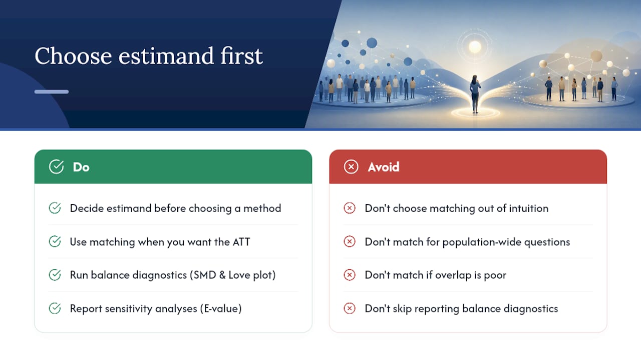
The most consistent mistake in applied PSM work is not a technical one. Researchers reach for matching because it feels intuitive, then work backward to justify the estimand. The correct sequence runs the other way: decide what causal question you are answering, identify the estimand that corresponds to it, then choose the method that targets that estimand.
Matching is the right tool when you genuinely want the ATT, when you have a well-defined treated population, and when the clinical or policy question is about the people who actually received treatment. It is the wrong tool when your question is population-wide, when overlap is poor, or when sample loss after matching would leave you with a matched set that no longer represents the treated group you care about.
The diagnostics are not a formality. An SMD table and a Love plot are the evidence that your matched groups are comparable. Skipping them, or running them and not reporting them, is the observational-study equivalent of not reporting randomization checks in an RCT. Sensitivity analyses are not optional either: every PSM result rests on the untestable assumption of no unmeasured confounding, and the E-value or Rosenbaum bounds are the honest acknowledgment of that limitation.
One practical recommendation: when you are uncertain whether to match or weight, run both, compare the balance diagnostics, and report both estimates. Convergence across methods is evidence of robustness; divergence is a signal worth investigating before you commit to a single answer.
Plotstudio runs your PSM workflow locally, with a full audit trail
Reproducible PSM analysis requires more than good code. It requires a workflow where the analysis plan is locked before execution, the data never leaves a secure environment, and every output is traceable back to the exact code and parameters that produced it.
Plotstudio is built for exactly this. Researchers connect their tabular data, and AI agents plan, code, and execute the full PSM pipeline in R or Python, including MatchIt, WeightIt, and cobalt workflows, on the researcher’s own machine. Data never touches a cloud server, which makes it viable for IRB-governed and HIPAA-covered datasets that cannot be uploaded to a general-purpose tool. Every analysis is gated behind a plan the researcher reviews and approves before any code runs, functioning as a pre-registration and an audit trail in one step.
The outputs Plotstudio produces for PSM analyses include annotated Jupyter notebooks, PDF reports with embedded Love plots and SMD tables, and permanent searchable analysis pages that supervisors, reviewers, and auditors can trace from result back to raw data. For research teams and institutions that need enterprise-grade reproducible analytics, Plotstudio’s local execution model and pre-registered analysis plans address the two requirements that general AI tools cannot meet. Start a free trial or explore the research partners program to see how it fits your lab’s workflow.
Sources
The references below are the canonical starting points for PSM theory, applied guidance, and software documentation.
- The central role of the propensity score in observational studies for causal effects
- Theory and practice of propensity score analysis - PMC
- Gking
- Propensity Score Analysis (Columbia Mailman School page)