One Command Reproducible Analysis Workflow for PhD Researchers

A reproducible analysis workflow bundles a machine-readable pipeline, a pinned computational environment, and a durable code deposit so another researcher can re-run your results exactly. Strip away any of those three layers and reproducibility collapses, no matter how tidy your script looks. Get all three right and you hand a reviewer, supervisor, or your own future self a package that actually runs.
TL;DR:
- Effective reproducible workflows require three layers: a machine-readable pipeline, a fixed computing environment, and a durable code deposit, all working together.
- Proper structuring includes separating raw, processed, and analysis-ready data, alongside detailed documentation and a manifest with checksums and version info.
- Using version control like Git, containerization such as Docker, and automation tools like Make or Snakemake ensures exact reruns and long-term access, especially for large datasets.
- Long-term reproducibility depends on depositing code and data in persistent repositories like Zenodo or Software Heritage, with proper licensing and citation files.
- Implementing provenance tracking for each result and establishing a simple, repeatable pipeline encourages lab-wide adoption and rapid, audit-ready verification.
Table of Contents
- What Are the Core Stages of a Reproducible Analysis Workflow?
- How Should You Structure a Research Compendium?
- Why Does Git Matter for Reproducible Data Analysis?
- How Do You Pin a Computational Environment for Reproducibility?
- Which Workflow Automation Tool Fits Your Project?
- How Do You Track Provenance for Every Reported Number?
- What Belongs in a Reproducible Code Review Checklist?
- How Should You Archive Code and Data for Long-Term Reuse?
- What Is a Minimal Reproducible Package, Step by Step?
- How PlotStudio Operationalizes a Reproducible Analysis Workflow
- What Privacy Steps Does Sensitive Data Require in a Reproducible Workflow?
- How Do You Manage Large Datasets and Storage in a Reproducible Pipeline?
- What Licensing and Legal Issues Affect Code and Data Sharing?
- Rolling Out Reproducible Workflows in a Real Lab
- Try PlotStudio for Your Next Reproducible Analysis
- Sources
What Are the Core Stages of a Reproducible Analysis Workflow?
Every reproducible analysis workflow moves through three stages, and the failure point is almost always the seams between them, not the stages themselves. Data acquisition, processing, and analysis/reporting each need a distinct artifact trail, or the chain of custody between your raw numbers and your published figure breaks somewhere nobody can find it later.
Data acquisition produces raw data, and raw data stays untouched. The moment you filter, recode, or merge it, you have created a derivative, and that derivative needs its own file, its own name, and its own place in the folder structure. Confusing “raw” with “analysis-ready” is the single most common reproducibility failure in academic projects, because six months later nobody remembers which spreadsheet was the original and which one had three rows quietly dropped for missing consent forms.
Data processing turns raw data into analysis-ready data, and this is where documentation earns its keep. A data dictionary that defines every variable, its units, and its allowed range does more to prevent silent errors than any amount of careful coding. Sample-selection logs matter just as much: if you excluded 40 participants for incomplete follow-up, that exclusion needs a timestamped record, not a comment buried in a script you’ll forget you wrote.
Data analysis and reporting is where dynamic documents like R Markdown and Quarto earn their place. They knit your code, your output, and your prose into a single file, so the number in your abstract is generated by the same code block a reviewer can inspect, not typed in by hand after eyeballing a console. That distinction between “computed” and “transcribed” is exactly what most manuscript-level reproducibility failures come down to.
A minimal template for this stage sequence looks like:
- Raw data: locked, read-only, accompanied by a source note (survey platform, scrape date, instrument version).
- Processing scripts: numbered in execution order (
01_clean.R,02_merge.R), each writing a clearly named output. - Analysis-ready data: a single file or set of files that every downstream analysis reads from, never modifies.
- Data dictionary: variable names, types, units, and any recoding logic, kept as a plain-text or spreadsheet file alongside the data.
- Dynamic report: an R Markdown or Quarto document that reads the analysis-ready data and renders both the manuscript prose and the figures from the same source.
This sequence matters because combining dynamic reporting with disciplined stage separation is what produces genuine computational reproducibility, rather than a document that merely looks reproducible until someone tries to run it on a different machine. The processing and analysis split also means a collaborator can swap in a corrected raw file and rerun everything without touching a single line of analysis code.
How Should You Structure a Research Compendium?
A research compendium is just a project folder organized so a stranger, or your own future self, can find every input, every step, and every output without asking you a question. The structure below works for most academic projects, from a single paper to a multi-chapter thesis.
- Root README stating the project’s purpose, the software required to run it, and the exact command that reproduces the main results.
data/split intoraw/(untouched) andprocessed/(analysis-ready), each with its own short README describing provenance.code/with numbered scripts or a single orchestrating script, plus any custom functions in asrc/orR/subfolder.results/for figures, tables, and model outputs, generated only by code, never edited by hand.MANIFEST.jsonat the root listing every tracked file’s hash, the run order, and the software versions used to generate it.
That manifest file does more work than its size suggests. A well-built one contains file checksums for the raw data (so you can detect silent corruption or accidental edits), the execution order of scripts, and the exact versions of R, Python, or key packages used for the run. A practical replication bundle includes a manifest alongside data, code, and environment files, enabling auditability. precisely so a reviewer, or an automated check, can confirm nothing has drifted since the paper was submitted.
Whether to formalize this as an actual R package or keep it as a plain folder depends on reuse. If you expect to reuse the analysis functions across multiple papers or hand them to labmates, wrapping them in an R package structure with DESCRIPTION and NAMESPACE files buys you dependency tracking and built-in documentation checks. For a single paper, a well-labeled compendium folder is usually enough, and structuring projects this way has been linked to higher citation counts and lower reentry costs when other researchers come back to extend the work later. The PlotStudio guide on PhD data analysis workflows walks through a compendium layout suited to dissertation chapters specifically, where you need several self-contained analyses inside one larger project.
Why Does Git Matter for Reproducible Data Analysis?
Version control turns a folder of scripts into a timestamped, auditable history, and Git is the tool academic reproducibility has settled on almost universally. Without it, “reproducible” analysis usually means a Dropbox folder with files named analysis_final_v3_USE_THIS.R, which is not reproducible at all.
A workable Git strategy for a publication project follows a few habits:
- Commit at the level of a single logical change (one bug fix, one new analysis step) rather than batching a week of work into one commit message.
- Tag the exact commit used to generate submitted results (
git tag v1.0-submission), so you can return to that precise state months later during peer review. - Use pull requests, even solo, to force a moment of self-review before merging a change into the main analysis branch.
- Keep a
CHANGELOG.mdnoting any deviation from a pre-registered analysis plan, with the commit hash where it happened.
Pull requests matter more in collaborative labs than solo projects, but the discipline transfers either way. A code review checklist, even a short one, catches the kind of logic error that reproducibility alone won’t: the practical recommendations from a large-scale review of epidemiological code emphasize systematic code review and comprehensible code as two of the highest-value habits for reducing silent analytical errors.
Continuous integration adds an automated layer on top of this. A CI pipeline, run through GitHub Actions or a similar service, can execute a smoke test on every push, confirming that your analysis script still runs end to end on a clean environment. It can also render your Quarto or R Markdown report automatically and attach the PDF as a build artifact, giving you a “build passing” badge that signals to reviewers the pipeline isn’t just present but actually functional.
Pro Tip: Set your CI job to run on a minimal, downsampled version of your data rather than the full dataset. A ten-row smoke test that fails in ninety seconds catches broken imports and renamed variables just as well as a full run that takes twenty minutes, and you’ll actually let it run before every commit instead of skipping it when you’re in a hurry.
How Do You Pin a Computational Environment for Reproducibility?
Lockfiles alone will not keep your analysis reproducible for more than a year or two, because they capture package versions without the underlying system libraries, compilers, and operating system quirks that those packages quietly depend on. Dynamic documents and dependency files are necessary but not sufficient for long-term reproducibility; the environment underneath them has to be captured too.
For R projects, renv snapshots the exact package versions your project used into a lockfile, and restoring that lockfile on another machine reinstalls precisely those versions. For Python, conda env export > environment.yml does the equivalent, capturing both Python packages and, in many cases, system-level dependencies that pip alone would miss. Both tools solve the “it worked on my laptop” problem for a colleague running the same operating system and architecture.
They stop solving it the moment someone runs your project on a different OS, a different chip architecture, or five years in the future when a system library your code depends on has been deprecated. That is what containerization is for. A minimal Dockerfile pattern for an R analysis looks something like this:
- Start from a versioned base image, such as
rocker/r-ver:4.3.1, neverlatest. - Copy your
renv.lockfile and restore it inside the container. - Copy your project code and data-processing scripts.
- Set the working directory and define the command that renders your final report.
The version pin in that first step matters more than it looks. Container tags like “latest” are mutable and will silently point to a different image months from now, which quietly breaks reproducibility even though your Dockerfile hasn’t changed a single line. Pinning by a specific image digest, not just a version tag, gives you a truly immutable reference.
Even a perfectly pinned container has limits. Floating-point behavior can vary across hardware, and parallelized code can introduce nondeterminism that survives inside an identical container, so bit-for-bit identical output across machines is not always achievable. Build a small-run verification step into your pipeline instead: rerun a subset of the analysis and check that results fall within a tight numerical tolerance, rather than demanding exact equality.
CASRAI’s synthesis of reproducibility infrastructure identifies three separable requirements: a machine-readable workflow, a captured environment, and a durable code identity. Environment pinning covers only the middle piece, and skipping the other two leaves your container sitting on a shelf nobody can find or run.
Which Workflow Automation Tool Fits Your Project?
The right automation tool depends on scale and execution target, not personal preference, and picking the wrong one wastes more setup time than it saves.
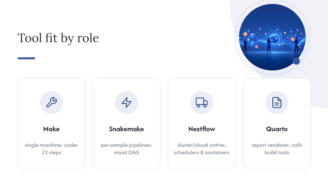
Make works well for a single-machine analysis with a handful of processing steps: clean data, fit model, render report. Its dependency logic is simple. Each target lists the files it needs and the files it produces, and Make only reruns steps whose inputs have changed, which saves real time during manuscript revisions when you tweak one figure and don’t want to rerun a two-hour model fit.
Snakemake scales better for projects with dozens of samples processed through the same steps, common in genomics or any field with per-subject pipelines. It expresses the same dependency logic as Make but generates an explicit directed acyclic graph (DAG) you can visualize, which makes debugging a broken pipeline far faster than tracing through nested shell scripts.
Nextflow targets high-performance and cluster computing, with native support for containerized execution steps and cloud or HPC schedulers. If your analysis needs to run on a university cluster or scale across cloud nodes, Nextflow’s execution model handles that natively where Make and Snakemake need extra tooling bolted on.
Quarto pipelines sit at a different layer. Quarto doesn’t replace a build tool. It orchestrates the rendering of your final report, and it composes well with any of the three above, calling Snakemake or Make as a preprocessing step before rendering the manuscript document itself.
A practical rule of thumb: use Make for a single-author paper with under a dozen processing steps, Snakemake once you have repeated per-sample logic across more than a handful of samples, and Nextflow once cluster or cloud execution enters the picture. Whichever you choose, wrap it inside a container and trigger it from your CI pipeline, so the DAG runs identically whether it executes on your laptop, a collaborator’s machine, or a GitHub Actions runner.
How Do You Track Provenance for Every Reported Number?
Provenance answers a question reviewers increasingly ask directly: where did this specific number come from? Without a lineage record, the honest answer is often “somewhere in a 400-line script,” which satisfies nobody.
A workable provenance record for each result captures a small, consistent set of fields:
- A run ID, generated automatically at execution time.
- A hash of the input data file used for that run.
- The exact parameters passed to the analysis function (model specification, random seed, subgroup filters).
- The function or script name that produced the output.
- A timestamp and the environment identifier (container digest or lockfile hash) active during the run.
Storing these fields in a lineage.json file next to your MANIFEST.json turns your replication package into something a reviewer, or an automated check, can query directly rather than reconstruct by reading code. A replication bundle built around a manifest and a lineage file, packaged with data, code, and environment material, enables exactly this kind of audit-grade tracing, because every reported figure can be traced back to the exact function call and inputs that generated it.
Spot-checking is where this pays off during peer review. A reviewer, or a journal’s reproducibility editor, can pick three numbers from your results table at random, look them up in lineage.json, rerun just those function calls, and confirm the outputs match, without rerunning your entire multi-hour pipeline. That is a far more realistic reproducibility check than expecting anyone to rebuild your whole analysis from scratch.
Pro Tip: Auto-generate lineage entries inside your analysis functions themselves, not as a separate manual logging step. A wrapper function that writes a lineage record every time it’s called costs almost nothing to build and never gets forgotten the way manual documentation does.
What Belongs in a Reproducible Code Review Checklist?
Reproducibility gets your code to run again. It does not guarantee the logic inside it is correct, and that gap is where a surprising number of published errors live. A short, disciplined review process closes it.
- Run a smoke test first. Before reviewing logic, confirm the code actually executes on a clean environment without errors. If it doesn’t run, nothing else about the review matters yet.
- Check readability before correctness. Can a second person follow the analysis steps without asking the author what a variable name means? Unclear code hides logic errors that clear code exposes on sight.
- Verify sample selection transparency. Every inclusion or exclusion criterion applied to the data should be visible in code or the sample-selection log, not buried in an unlogged manual filter.
- Confirm stated assumptions match the code. If the analysis plan says “linear mixed-effects model with random intercepts by site,” the code should implement exactly that, not a simplified variant nobody flagged.
- Log any deviation from the pre-registered plan. If a robustness check led you to switch models or drop an outlier, that deviation belongs in the
CHANGELOG.mdwith a commit hash and a one-line justification, not a silent edit.
Unit tests for individual analysis functions add another layer of protection cheaply. A function that computes a hazard ratio, for instance, can be tested against a small synthetic dataset with a known expected output. If a later refactor breaks the function, the test catches it before the error reaches a manuscript draft, rather than after a reviewer notices the numbers don’t match your supplementary tables.
A review of reproducibility practices in medical research found that systematic code review, comprehensible code, and transparent reporting of decisions were among the highest-value, lowest-cost interventions available to researchers, ranking above more elaborate infrastructure investments for catching the errors that actually make it into print.
How Should You Archive Code and Data for Long-Term Reuse?
A GitHub repository is not a permanent archive. Repositories get deleted, accounts lapse, and organizations restructure, so durable reproducibility needs a deposit outside the platform where you did the day-to-day work.
Zenodo issues a DOI for your code and data deposit, which makes the release citable in your manuscript’s methods section, exactly like a dataset or a paper. Connecting your GitHub repository to Zenodo lets every tagged release generate a new, permanent DOI automatically, so your v1.0-submission tag from earlier becomes a citable, permanent snapshot the moment you push it.
Software Heritage takes a different but complementary approach, archiving source code at the level of individual files and content-addressed objects rather than issuing a single citable DOI per release. Durable archival through both DOI-based deposits and content-addressed archives is what preserves reproducibility over time, since Zenodo protects against your specific release disappearing while Software Heritage protects against the broader ecosystem of dependencies and forks vanishing.
Preparing a release for either platform takes a handful of concrete steps:
- Add a
CITATION.cfffile at the repository root, specifying how you want the code cited, including author names, ORCID IDs, and the version. - Choose an explicit license (MIT or GPL for code, CC BY for data and documentation) rather than leaving the repository unlicensed, which legally defaults to “all rights reserved” even on a public GitHub page.
- Tag the release commit, connect the repository to Zenodo, and confirm the automated DOI minting completes before submitting your manuscript.
- For computationally expensive analyses, deposit intermediate results alongside raw data, and include a small-scale verification script that reruns a subset of the pipeline in minutes rather than hours, so reviewers can validate the logic without needing your original compute budget.
What Is a Minimal Reproducible Package, Step by Step?
A minimal reproducible package should let a stranger run one command and get your results back. That’s the bar. If your pipeline needs an email to you explaining which script to run first, it isn’t reproducible yet.
A practical one-command build, using Make as the orchestrator, looks like:
make all
That single command should trigger data processing, run the analysis scripts in order, render the final Quarto or R Markdown report, and output a complete artifact set: analysis-ready data, figures, tables, the rendered PDF, and a MANIFEST.json confirming what was produced and when.
Adopting the full stack at once is unrealistic for most researchers mid-project, so prioritize by effort against payoff:
- Low effort, start today: write a README with the exact commands to reproduce your results, and separate raw data from processed data into distinct folders.
- Low to medium effort: commit your project to Git, tag the version used for your submission, and add a data dictionary.
- Medium effort: snapshot your environment with renv or conda, and add a
CITATION.cfffile plus an explicit license. - Medium to high effort: containerize with Docker, pinning by digest, and wrap your pipeline in Make or Snakemake.
- High effort, highest payoff: add per-result provenance logging, deposit a tagged release to Zenodo and Software Heritage, and set up CI to smoke-test the pipeline on every push.
For computationally expensive analyses, always save intermediate results rather than only the final output, and build a small verification run using a downsampled dataset that completes in minutes. A reviewer checking your reproducibility package almost never has your original compute budget, and a fast verification path is often the difference between a package that gets checked and one that gets waved through unread.
| Effort Level | Action | Reproducibility Gain |
|---|---|---|
| Low | README with exact run commands, raw/processed data separation | Prevents most “which file is which” confusion |
| Low to medium | Git commit history, version tagging, data dictionary | Creates an auditable project history |
| Medium | Environment lockfile (renv/conda), CITATION.cff, explicit license | Makes the environment and reuse terms explicit |
| Medium to high | Docker container pinned by digest, Make/Snakemake automation | Removes “works on my machine” failures |
| High | Per-result provenance, Zenodo/Software Heritage deposit, CI smoke tests | Enables audit-grade, spot-checkable verification |
How PlotStudio Operationalizes a Reproducible Analysis Workflow
Some agentic analytics platforms are built around the same three-layer requirement this article has walked through: workflow logic, a pinned environment, and a durable, checkable record of what ran. Typically, every analysis there starts with an analysis plan a researcher reviews and approves before any code executes, stating methods, assumptions, and success criteria up front. Such a plan functions as a pre-registration and an audit trail in one document, which maps directly onto the code-review and provenance habits covered above.
Some research-grade analytics platforms run analysis locally on the researcher’s own machine, which matters specifically for IRB-governed, NHS, or GDPR special-category data that cannot legally leave the device for a cloud tool to process. They run both R and Python natively and cover methods academic work actually needs, including survival analysis, Cox proportional hazards, mixed-effects models, and multiple-comparison correction, so users don’t have to translate between two ecosystems mid-project.
Some platforms let a lab encode its own required steps, statistical thresholds, and forbidden shortcuts once, so every subsequent analysis follows that discipline’s methodology automatically rather than a generic default. When an analysis finishes, these platforms typically export a full reproducibility package: annotated notebooks, a PDF report, and a permanent, searchable analysis page, giving a supervisor or peer reviewer a direct trace from raw data to reported figure.
A reasonable first step is importing a sample dataset, running a template analysis close to your own study design, and exporting the resulting replication package to see the audit trail firsthand.
What Privacy Steps Does Sensitive Data Require in a Reproducible Workflow?
Reproducibility and data privacy pull in opposite directions by default. Reproducibility wants every input shared; IRB and GDPR rules on human-subjects data want the opposite. The resolution isn’t to skip reproducibility on sensitive projects. It’s to reproduce the pipeline while protecting the data.
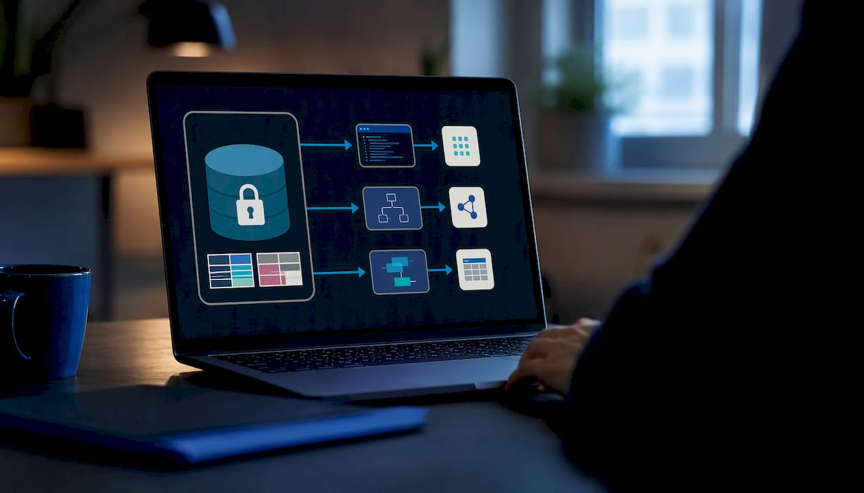
Start by never committing raw identifiable data to Git, even in a private repository. History persists indefinitely, and a single accidental commit of a file with names or dates of birth is effectively permanent. Keep raw sensitive data outside version control entirely, referenced by path in your scripts rather than stored inside the repository.
For sharing purposes, generate a synthetic or de-identified version of your dataset that preserves the statistical structure without the disclosure risk. Publish your code and pipeline against that synthetic version, so a reviewer can verify your logic runs correctly, even without access to the real data. Document exactly which fields were removed or perturbed, and where, in your data dictionary.
Where a data use agreement legally requires local-only processing, running your entire pipeline on a machine that never uploads data to a cloud service isn’t optional. This is precisely the constraint that makes local execution, rather than a browser-based analysis tool, the only workable choice for IRB-governed patient data, and it should shape your tool selection well before you start writing analysis code.
How Do You Manage Large Datasets and Storage in a Reproducible Pipeline?
Large datasets break the “commit everything to Git” habit that works fine for small projects. Git handles text diffs well; it handles multi-gigabyte binary files badly, bloating repository size and slowing every clone to a crawl.
Git-LFS (Large File Storage) solves the immediate problem by storing large binary files outside the main Git history while keeping a lightweight pointer inside your repository, so cloning stays fast even with large raw datasets tracked alongside your code. For datasets running into the hundreds of gigabytes or beyond, a dedicated data repository, whether an institutional server or a cloud storage bucket, makes more sense than Git-LFS, with your code referencing a stable download path or API endpoint rather than storing the data directly.
Whatever storage layer you choose, record the exact retrieval method in your README: the URL, the access credentials process, and the expected file size and checksum after download. That checksum check matters more than it sounds. A corrupted or partial download of a 40GB dataset can produce plausible-looking results that are subtly wrong, and a hash comparison against your MANIFEST.json catches that before it reaches your analysis.
For genuinely large-scale computation, budget for intermediate result caching. Save the output of expensive steps, like a model fit that takes six hours, to disk rather than recomputing it on every pipeline rerun, and let your workflow manager’s dependency logic decide when a rerun is actually necessary.
What Licensing and Legal Issues Affect Code and Data Sharing?
An unlicensed public repository is not automatically open for reuse. Under default copyright law, no explicit license means “all rights reserved,” even when the code sits publicly on GitHub, which surprises a lot of researchers who assumed public visibility implied permission to reuse.
Pick a license deliberately rather than skipping the decision. MIT and Apache 2.0 are permissive choices for code, allowing reuse with minimal restriction beyond attribution. GPL requires derivative works to also be open source, which some labs prefer for philosophical reasons but which can complicate collaboration with industry partners. For data and documentation specifically, a Creative Commons license, most commonly CC BY, is the standard choice across academic fields.
Data licensing carries additional legal weight beyond code. If your dataset includes any personally identifiable information, no license can override the underlying legal restrictions from your IRB approval or data use agreement; the license governs your original contribution, not the underlying subjects’ privacy rights. Journals increasingly require a data availability statement specifying exactly what can be shared and under what terms, so resolve licensing before submission, not after a reviewer asks.
Institutional policies sometimes claim ownership over code and data produced under a grant, which can restrict what you’re legally able to license publicly at all. Check your institution’s technology transfer or research policy office before defaulting to an open license, particularly if the work was funded by an agency with its own data-sharing mandates.
Rolling Out Reproducible Workflows in a Real Lab
Getting a lab to actually adopt reproducible workflows is a culture problem dressed up as a technical one. Nobody adopts a new practice because a guide told them to. They adopt it because the friction of starting is low and the payoff shows up fast enough to notice.
Start with one small, visible win rather than a lab-wide mandate. Build a single Quarto template for the most common analysis type in your group, automate that one pipeline end to end, and put a lightweight code-review rota in place where two people glance at each other’s scripts before a result goes into a draft. That’s enough to establish the habit without asking anyone to learn five new tools simultaneously.
Incentives decide whether it sticks. A lab-wide research compendium that labmates can actually reuse, credit given explicitly for producing a clean, reproducible analysis (not just for the paper it supported), and a supervisor who asks “can I rerun this?” during lab meetings, do more to shift behavior than any documentation ever will. The biggest barrier to reproducibility adoption is rarely technical skill. It’s a lack of incentive structures rewarding the extra effort, and that has to be solved at the lab level, not the individual one.
The payoff that eventually sells skeptics is almost always selfish, and that’s fine. Six months after submission, when a reviewer asks for a new subgroup analysis, a reproducible pipeline turns that request into an afternoon’s work instead of a week spent reconstructing what you did the first time.
— Aymen
Try PlotStudio for Your Next Reproducible Analysis
PlotStudio maps directly onto the checklist covered throughout this piece: local execution for IRB-governed and GDPR-restricted data, a gated analysis plan that doubles as your provenance record, and an exportable reproducibility package that gives reviewers exactly the audit trail they now expect. Where a general AI chart tool leaves you rebuilding lockfiles, manifests, and lineage tracking by hand, PlotStudio produces the annotated notebook, PDF report, and searchable analysis page automatically, every time an analysis runs.
For researchers weighing PlotStudio against a general-purpose analysis assistant, the advanced data analysis alternative comparison breaks down exactly where a research-grade platform earns its keep over a generic chatbot wrapper. If you’re currently building compendiums by hand, the reproducibility guide for analysts is worth reading alongside your first PlotStudio project. For labs training new graduate students on these habits, AmmarAI’s guide to AI-assisted student workflows covers the adoption side well.
A practical next step: import a sample dataset into a research-grade analytics platform, run an analysis template against it, and export the resulting replication package to see the full audit trail before committing your first real study to the workflow.
Sources
For deeper technical grounding beyond this guide, a handful of sources cover the infrastructure and practice in more depth. CASRAI’s reproducibility infrastructure guide lays out the workflow, environment, and identity framework referenced throughout this article. Peikert et al.'s tutorial walks through a full R Markdown, Git, Make, and Docker pipeline with runnable examples. The Rotterdam Study review offers a concrete code-review checklist drawn from epidemiological research. Poldrack’s Stanford open science guide and the StatsPAI replication workflow guide round out the practical side, alongside official documentation for Quarto, renv, Docker, Snakemake, and Zenodo.
- Reproducibility infrastructure, workflows, containers, code sharing — CASRAI
- A reproducible data analysis workflow with R Markdown, Git, Make, and Docker — Peikert et al.
- Practical recommendations to improve reproducibility of code — Rotterdam Study review
- Replication workflow — StatsPAI