Sample Size Determination: A Practical Guide for Researchers

The sample size you need is the smallest n that meets your precision or power target after accounting for design effects and expected losses. That single principle drives every calculation in this guide. Whether you are planning a clinical trial, a survey, or a behavioral experiment, sample size determination covers two distinct objectives: estimation (how narrow does your confidence interval need to be?) and hypothesis testing (how likely are you to detect a real effect?). Nail the objective first, then work through these five steps before you open any calculator:
- Set your objective. Decide whether you are estimating a parameter with a target margin of error or testing a hypothesis with a target power level.
- Define your effect size or precision target. Choose the minimum difference or precision that is practically meaningful, not just statistically convenient.
- Choose alpha and power (or confidence level and margin of error). Standard defaults are alpha = 0.05 and power = 0.80, but your field or IRB may require stricter thresholds.
- Select the right formula or software and run the calculation. G*Power covers most standard test families; Power offers interactive web-based sensitivity graphs; Calculator handles quick proportion checks.
- Inflate for nonresponse, attrition, or clustering. Add 10–20% for surveys, adjust by the design effect (DEFF) for cluster samples, and account for expected dropout in longitudinal work.
Key Takeaways
Accurate sample size determination requires defining your objective, effect size, alpha, power, and variability before running any calculation, then inflating the result for expected losses and design complexity.
| Point | Details |
|---|---|
| Choose your objective first | Decide between margin-of-error estimation and power-based hypothesis testing before selecting any formula. |
| Justify the effect size | Ground the minimum detectable effect in prior literature, pilot data, or a field-specific MCID, not Cohen’s generic conventions. |
| Adjust for design complexity | Multiply by DEFF = 1 + (m−1) × ICC for clustered designs; a modest ICC of 0.05 with clusters of 20 nearly doubles the required n. |
| Inflate for losses | Divide required n by the expected response or retention rate (e.g., n / 0.80 for 20% attrition) before finalizing recruitment targets. |
| Plotstudio for reproducibility | Plotstudio’s local, gated workflows store sample-size calculations in a permanent audit trail suitable for IRB and peer-review scrutiny. |
Table of Contents
- Why sample size determination matters for your study
- What inputs do you need before calculating n?
- Core formulas and how to apply them
- How to run an a priori power analysis step by step
- Which calculators and software should you use?
- How do complex designs change your required sample size?
- How do you adapt your sample size to real-world constraints?
- Common mistakes in sample-size planning and how to avoid them
- Making your sample-size plan reproducible and defensible
- The tradeoffs researchers actually face
- Plotstudio brings reproducible sample-size planning into your research workflow
- Sources
Why sample size determination matters for your study
Sample size is the number of observations or units required to achieve a prespecified statistical objective. Too few, and you risk missing a real effect entirely. Too many, and you waste resources and, in clinical or social research, expose participants to unnecessary burden.
The consequences of underpowering are concrete. A study with insufficient n inflates the Type II error rate (failing to detect a true effect), and any effect it does detect is likely to be an overestimate of the true population value. Journals and grant reviewers increasingly flag underpowered studies as a credibility risk, not just a methodological footnote. On the other side, an oversized study consumes budget, extends timelines, and in trials involving human subjects, raises ethical concerns about enrolling more participants than the science requires.
Two frameworks govern the calculation. Larger sample sizes narrow the sampling distribution and increase power, but the relationship is nonlinear. Doubling power from 0.50 to 0.80 requires far fewer additional subjects than pushing from 0.80 to 0.95.
Cohen’s power conventions (small d = 0.2, medium d = 0.5, large d = 0.8) are widely cited but frequently misapplied. They were calibrated to social science data from the 1960s and carry no guarantee of practical relevance in your field. Use them as a rough orientation, not as a substitute for a domain-specific justification.
What inputs do you need before calculating n?
Every sample size formula is a function of the same core parameters. Get these right, and the arithmetic is straightforward.
- Objective. Test or estimate? This determines which formula family applies.
- Effect size. The minimum difference or association you need to detect. For means, this is often expressed as Cohen’s d (the difference divided by the pooled SD). For proportions, it is the absolute or relative difference between two rates.
- Alpha (Type I error rate). The probability of a false positive. Conventional default: 0.05. Regulatory or safety contexts often require 0.01 or lower.
- Power (1 − beta). The probability of detecting a true effect. Conventional minimum: 0.80. Many journals and NIH grant reviewers now expect 0.90 for primary outcomes.
- Variability. The standard deviation for continuous outcomes, or the baseline proportion for binary outcomes. This is the parameter researchers most often underestimate.
- Allocation ratio. The ratio of subjects in each group. Equal allocation (1:1) is most efficient; unequal ratios increase total n required.
- Expected loss. Anticipated dropout, nonresponse, or exclusion rate. Always plan for it explicitly.
- Population size. Matters only when the population is small relative to the sample (finite population correction applies roughly when n exceeds 5% of N).
- Multiple comparisons and subgroup plans. Each additional test inflates the family-wise error rate. Bonferroni correction or false discovery rate (FDR) adjustment increases required n per comparison.
How to choose your effect size
The most defensible approach is to anchor the effect size in prior literature or a pilot study. Search for published SDs and mean differences in studies using the same outcome measure and population. If none exist, use a pilot study of 20–30 subjects to estimate variability, then apply a conservative (larger) SD in your main calculation to avoid optimistic inflation. The minimum clinically important difference (MCID) or minimum practically important difference (MPID) is the right target when your field has established one.
Avoid picking Cohen’s “medium” effect simply because it is the default in a tutorial. A medium effect in psychology (d = 0.5) translates to a very different biological or educational reality than a medium effect in pharmacology.
Estimating variability
Published SDs from similar studies are the first choice. For proportions, the variance is maximized at p = 0.5, so using 0.5 as a conservative plug-in is standard practice when the true rate is unknown.
Pro Tip: Always plan for nonresponse or attrition by inflating your calculated n before finalizing recruitment targets. For longitudinal studies, model retention at each wave and compound the losses across time points.
Core formulas and how to apply them
The formulas below cover the four most common scenarios. All assume simple random sampling; adjustments for clustering and stratification appear in a later section.
A. Single proportion, margin-of-error approach
$$n = \frac{z_{\alpha/2}^2 \cdot \hat{p}(1-\hat{p})}{B^2}$$
At the conservative p̂ = 0.5 and B = 0.05, this yields n ≈ 385 for large populations, the standard result for a 95% CI with a ±5% margin. The NIST/SEMATECH e-Handbook provides full derivations for this and related precision-based formulas.
B. Single mean, margin-of-error approach
$$n = \frac{z_{\alpha/2}^2 \cdot \sigma^2}{B^2}$$
Here σ is the population (or estimated) standard deviation and B is the target half-width of the confidence interval. Use z when σ is known or the sample is large; switch to the t distribution when σ is estimated from a small sample (the formula becomes iterative because the t critical value depends on degrees of freedom, which depend on n).
C. Two-sample difference in means, power-based
$$n_{per\ group} = \frac{2\sigma^2(z_{\alpha/2} + z_\beta)^2}{\delta^2}$$
Where δ is the minimum detectable difference, σ is the common within-group SD, z_α/2 = 1.96 (two-tailed, alpha = 0.05), and z_β = 0.842 (power = 0.80). Always round up to the next integer.
D. Two-sample difference in proportions, power-based
$$n_{per\ group} = \frac{(z_{\alpha/2}\sqrt{2\bar{p}(1-\bar{p})} + z_\beta\sqrt{p_1(1-p_1)+p_2(1-p_2)})^2}{(p_1-p_2)^2}$$
Where p̄ = (p₁ + p₂)/2. This formula is more sensitive to the baseline rate than the means formula, so always check n at both the expected and a pessimistic baseline proportion.
Worked example 1: Estimating a proportion
A public health researcher wants to estimate the prevalence of hypertension in a county.
n = (1.96² × 0.5 × 0.5) / 0.03² = (3.8416 × 0.25) / 0.0009 = 0.9604 / 0.0009 ≈ 1,068
Worked example 2: Two-sample t-test (power-based)
A psychologist compares a new intervention to a control on a continuous outcome.
n per group = 2 × (1.96 + 0.842)² / 0.5² = 2 × 7.849 / 0.25 = 63 per group (126 total)
G*Power returns the same result for this configuration, confirming the manual calculation.
Which formula fits your study goal?
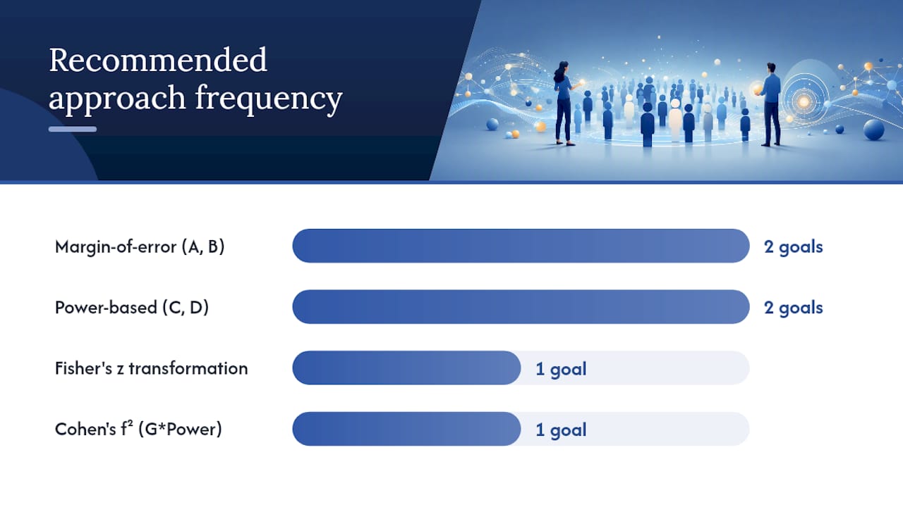
| Study goal | Outcome type | Recommended approach |
|---|---|---|
| Estimate a single proportion | Binary | Margin-of-error formula A |
| Estimate a single mean | Continuous | Margin-of-error formula B |
| Compare two independent groups | Continuous | Power-based formula C |
| Compare two independent groups | Binary | Power-based formula D |
| Test a correlation | Continuous | Fisher’s z transformation approach |
| Detect a regression coefficient | Continuous | Cohen’s f² approach via G*Power |
How to run an a priori power analysis step by step
A priori power analysis means you fix the inputs before collecting data and solve for n. This is the only defensible approach for grant applications and preregistrations. Post-hoc power calculated from observed data is circular and should never be used to explain a nonsignificant result.
- Confirm the primary test and analytic model. A two-sample t-test, a chi-square test, a mixed-effects model, and a Cox regression each require different power formulas. Locking the model first prevents formula mismatches.
- Specify the effect size and its source. State the minimum meaningful difference, the SD or baseline proportion, and where those numbers come from (published study, pilot data, or MCID from the literature).
- Choose alpha and target power. Document the rationale. If your IRB or funding agency specifies thresholds, use those; otherwise, alpha = 0.05 and power = 0.80 are the conventional minimums.
- Set the allocation ratio. Equal groups (1:1) maximize power for a given total n. If unequal allocation is required (e.g., 2:1 control-to-treatment), adjust the formula accordingly.
- Compute n using the appropriate formula or tool. For standard tests, G*Power is the most widely validated option across social, behavioral, and biomedical sciences. For quick web-based checks, power.statisticalcomputing.org returns the required n and plots the power curve simultaneously.
- Run sensitivity checks. Vary the effect size and SD across a plausible range and record the resulting n values. The table below illustrates this for the two-sample t-test example.
- Inflate for losses and practical constraints. Divide the required n by the expected retention or response rate, then round up.
Sensitivity check: required n per group (two-sample t-test, alpha = 0.05, power = 0.80)
Plotting this curve rather than reading a single row reveals that n is highly sensitive to effect size at the small-to-medium range. A researcher who assumes d = 0.5 but whose true effect is d = 0.3 will be severely underpowered with 64 subjects per group.
Which calculators and software should you use?
The right tool depends on your test family, your comfort with code, and whether you need a reproducible record of the calculation.
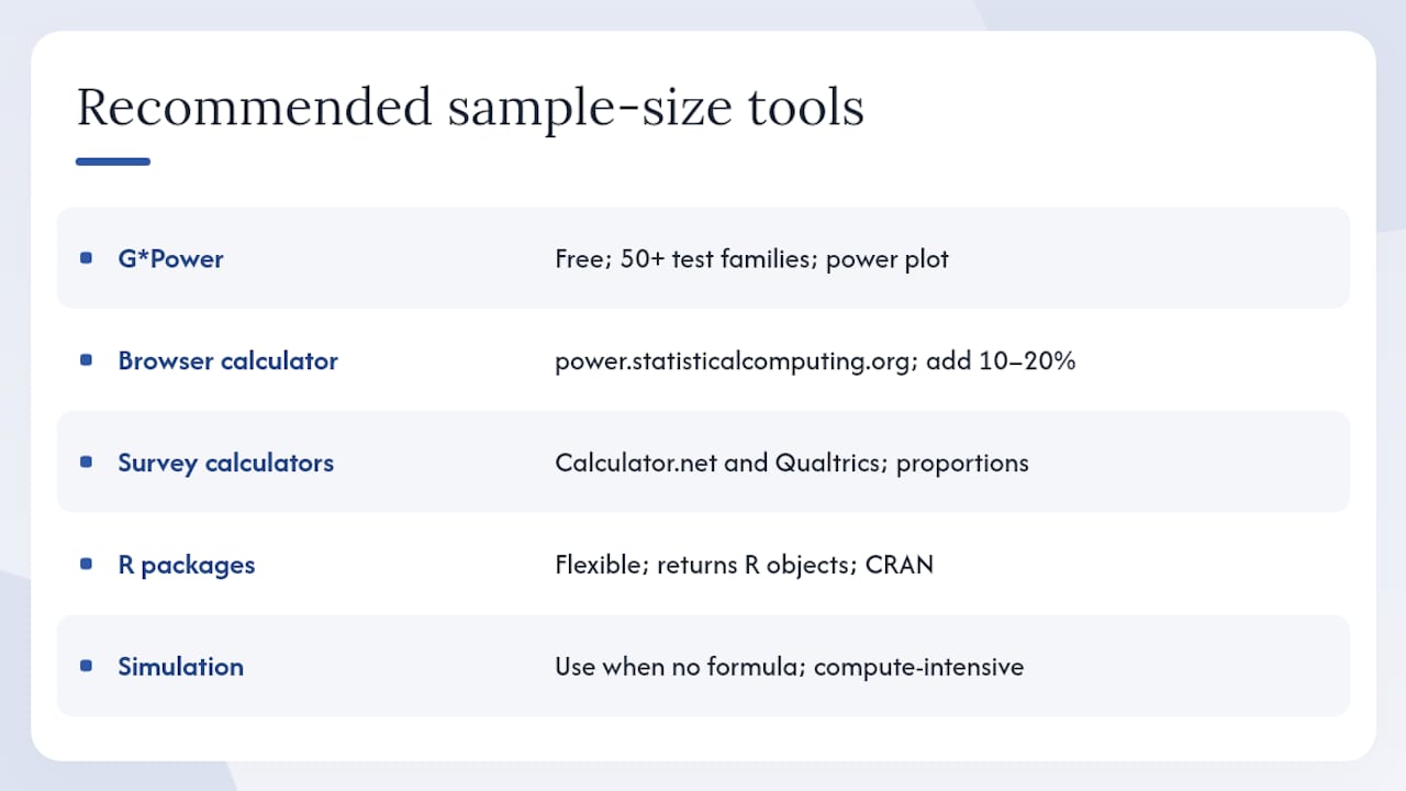
G*Power (free, Windows and macOS) is the standard choice for most researchers. It covers more than 50 test families, including t-tests, ANOVA, chi-square, correlation, regression, and several nonparametric tests. The interface walks you through specifying effect size, alpha, power, and allocation ratio, then returns n with a power plot. G*Power is particularly well-suited for social and behavioral science designs and is the tool most reviewers and IRBs recognize by name.
power.statisticalcomputing.org is a browser-based calculator that computes sample size, power, and effect size interchangeably and generates sensitivity graphs on the fly. It recommends adding 10–20% to the computed n to cover potential dropouts, which is a useful built-in reminder. No installation required, and the output is easy to screenshot for a preregistration.
Calculator.net and the Qualtrics sample size calculator are the fastest options for proportion-based survey planning. Both use the standard margin-of-error formula and are appropriate for quick feasibility checks, though neither handles complex designs or power-based calculations for comparative studies.
R packages give you the most flexibility and the most reproducible output. The pwr package covers the same test families as G*Power and returns results as R objects you can embed directly in an R Markdown or Quarto document. For clustered designs, clusterPower implements sample-size calculations for cluster-randomized trials, including ICC-based adjustments. Both packages are available on CRAN and install with a single command.
Simulation is the right approach when no closed-form formula exists: complex mixed models, non-normal outcomes, or nonstandard estimands. SAS documents simulation workflows for empirical power, and the same logic applies in R using replicate() or the simr package for mixed models. The tradeoff is computation time and the need to specify a full data-generating model, but simulation is often more accurate than analytic approximations for irregular designs.
Caveat: Every calculator embeds assumptions. G*Power assumes normality and equal variances for t-tests. Web calculators for proportions assume simple random sampling. Before treating any computed n as final, verify that the calculator’s assumptions match your study design.
How do complex designs change your required sample size?
Simple random sampling formulas underestimate n whenever your design introduces clustering, stratification, or repeated measures. Ignoring these adjustments is one of the most common and consequential errors in sample-size planning.
Clustering and the design effect
When subjects are sampled within clusters (schools, clinics, households), observations within the same cluster are correlated. The design effect (DEFF) quantifies how much this correlation inflates the required n relative to simple random sampling:
DEFF = 1 + (m − 1) × ICC
Where m is the average cluster size and ICC is the intraclass correlation coefficient. The adjusted sample size is:
n_adj = n_simple × DEFF
For example, if a simple random sample requires 200 subjects, clusters average 20 students each, and ICC = 0.05:
DEFF = 1 + (20 − 1) × 0.05 = 1 + 0.95 = 1.95
n_adj = 200 × 1.95 = 390 subjects (roughly double the unadjusted estimate)
NIH provides calculators and stepwise guidance for cluster-randomized and stepped-wedge trial designs, including ICC-based adjustments and variance component specification. The clusterPower R package handles the same calculations programmatically.
Stratified sampling
Stratification on a variable correlated with the outcome reduces variance and can lower total n relative to simple random sampling. Neyman allocation (allocating subjects to strata proportional to stratum size times stratum SD) achieves the minimum variance for a given total n. When strata SDs differ substantially, Neyman allocation can meaningfully reduce the required total compared to proportional allocation.
Repeated measures and longitudinal designs
Within-subject correlation is an asset in repeated-measures designs: it reduces the residual variance and therefore the required n per subject. The required sample size decreases as the within-subject correlation increases, but you must supply a credible estimate of that correlation (from pilot data or the literature) to avoid optimistic projections. Mixed-effects model power calculations require specifying both the fixed-effect structure and the variance-covariance matrix of the random effects. The simr package in R handles this via simulation when analytic formulas are unavailable.
Survival and time-to-event outcomes
Sample size for survival analyses is driven by the number of events, not the number of subjects enrolled. The required number of events depends on the hazard ratio, the target power, and alpha. Total enrollment then depends on the expected event rate and follow-up duration. For stepped-wedge and cluster-randomized time-to-event designs, NIH calculators and specialized R packages provide the most reliable estimates.
| Design type | Key adjustment | Primary tool |
|---|---|---|
| Cluster-randomized trial | Multiply by DEFF = 1 + (m−1) × ICC | NIH calculators, clusterPower ® |
| Stratified random sample | Apply Neyman allocation across strata | Standard formulas, NIST handbook |
| Repeated measures | Reduce variance by within-subject correlation | simr ®, G*Power repeated-measures module |
| Survival / time-to-event | Calculate required events, then back-calculate enrollment | NIH calculators, nQuery, specialized R packages |
How do you adapt your sample size to real-world constraints?
The ideal n from a formula and the n you can actually recruit are rarely the same number. Bridging that gap requires explicit, documented decisions rather than silent compromises.
Inflating for nonresponse and attrition
The standard adjustment is straightforward: divide the required n by the expected retention or response rate.
Example: A longitudinal study requires 150 completers at the final wave. Required enrollment: 150 / 0.70 = 215 participants at baseline.
For surveys, if the required completed responses is 385 and the expected response rate is 60%, recruit from a pool of at least 385 / 0.60 = 642 contacts. Web calculators at power.statisticalcomputing.org build this adjustment into their output.
When to run a pilot study
A pilot study of 20–40 subjects is worth the investment when the primary outcome’s SD is genuinely unknown and no published estimate is available. Use the pilot SD conservatively: add one standard error to the pilot estimate before plugging it into the main calculation. Never use the pilot effect size as the target for the main study’s power calculation. That practice inflates the expected effect and produces an underpowered main study.
- Pilot studies are also useful for estimating recruitment rates, refining eligibility criteria, and testing data collection procedures.
- Document pilot results separately from the main study preregistration so reviewers can assess the basis for your variance estimate.
- If the pilot SD is substantially larger than expected, revise the main-study n upward before opening enrollment.
Sequential and group-sequential designs
Group-sequential designs allow planned interim analyses with pre-specified stopping rules, which can reduce the average sample size when effects are large. The tradeoff is a more complex alpha-spending function (O’Brien-Fleming or Pocock boundaries are the standard options) and additional regulatory or IRB documentation. For most academic studies, a single planned interim look with a conservative alpha spend (e.g., spending 0.01 at interim and 0.04 at final) is manageable without specialized software.
Pro Tip: Before finalizing your recruitment target, run a feasibility check: estimate the number of eligible subjects in your target population, the expected screening-to-enrollment ratio, and the time required to reach your inflated n. If the timeline exceeds your study window, consider multi-site recruitment or a sequential design rather than silently reducing n below the power threshold.
Common mistakes in sample-size planning and how to avoid them
Most sample-size errors fall into a small number of recurring patterns. Recognizing them before submission is far less painful than addressing them during peer review.
Using post-hoc power to explain a null result. Retrospective power calculated from the observed effect size is circular: it is mathematically equivalent to reporting the p-value in a different format and adds no information about whether the study was adequately powered. Perform a priori power analysis before data collection and report that calculation, not a post-hoc version.
Relying on Cohen’s generic conventions without context. Labeling an effect as “medium” and plugging in d = 0.5 without a domain-specific justification is a red flag for reviewers. The minimum effect size should be grounded in prior literature, a pilot study, or an MCID established in your field.
Ignoring ICC for clustered designs. A study that treats clustered data as if it were a simple random sample will be systematically underpowered. Even a modest ICC of 0.05 with clusters of 20 nearly doubles the required n, as the worked example above shows.
Forgetting multiple-comparison adjustments. Each additional primary outcome or subgroup comparison inflates the family-wise Type I error rate. Bonferroni correction divides alpha by the number of comparisons; FDR methods (Benjamini-Hochberg) are less conservative for exploratory analyses. Either way, the adjusted alpha increases the required n per comparison.
Treating default calculator settings as universal truth. Most web calculators default to two-tailed tests, equal allocation, and simple random sampling. If your design is one-tailed, unequal, or clustered, those defaults produce the wrong n.
Pre-submission checklist
Before locking your sample size, verify each of the following:
- Correct test family selected and matched to the analytic model
- Effect size justified with a named source (published study, pilot data, or MCID)
- SD or baseline proportion sourced and documented
- Alpha and power choices stated with rationale
- Clustering or stratification adjustments applied where relevant
- Multiple-comparison correction applied if more than one primary test is planned
- Realistic response/retention rate used for inflation
- Calculation is reproducible (code, calculator output, or formula with inputs saved)
Treat the computed n as a minimum. Round up, never down, and document the rounding.
Making your sample-size plan reproducible and defensible
A sample-size calculation that cannot be reproduced by a reviewer is nearly as problematic as one that was never done. Preregistration and audit trails are now expected by most high-impact journals and NIH study sections.
What to record in a preregistration
A complete preregistration entry for sample size should include: the primary outcome and its scale, the minimum effect size and its justification, the estimated SD or baseline proportion and its source, the chosen alpha and power, the analytic model, the complete calculation (formula with inputs or saved calculator output), the expected loss rate and the inflated n, and any decision rules for interim analyses. Open Science Framework (OSF) and AsPredicted both support structured preregistration templates that cover these elements.
Versioned code and audit trails
If you calculate n in R, save the script in your project repository with a timestamp and a comment block that records the date, the study name, and the version of the pwr or clusterPower package used. If you use G*Power, export the protocol file (.gpp) and save a PDF of the output screen. For web calculators, a dated screenshot with the URL and all input values visible is sufficient for most IRB submissions.
Pro Tip: Lock the sample-size calculation in your preregistration or repository before data collection begins. Reviewers and IRBs increasingly request the original calculation file, not just the reported n. Plotstudio’s AI for academic research workflows gate every analysis behind a pre-approved plan, creating a permanent, searchable audit trail that satisfies this requirement without extra documentation overhead.
The SAS documentation on power and sample-size analysis notes that prospective analysis optimizes study design, and simulation is a viable alternative for unsupported models. The same principle applies to reproducibility: a prospective, documented calculation is the only version that holds up under scrutiny.
The tradeoffs researchers actually face
Balancing statistical ideals against recruitment realities is where sample-size planning gets genuinely hard. The right answer is rarely the textbook answer.
Different disciplines carry different norms. In clinical pharmacology, 0.90 power for a primary efficacy endpoint is often a regulatory expectation. In educational psychology, 0.80 is widely accepted, and effect sizes below d = 0.3 are rarely pursued because the practical significance is marginal even when statistical significance is achievable. Knowing your field’s conventions matters as much as knowing the formula.
What I find consistently underappreciated is the value of transparent justification over perfect precision. Reviewers can engage with a documented tradeoff. They cannot engage with a number that appears without context.
For researchers navigating these decisions across disciplines, Plotstudio’s statistical analysis methodology guide covers how analytic model choice connects back to sample-size requirements, which is a link that textbooks often leave implicit.
Plotstudio brings reproducible sample-size planning into your research workflow
Calculating the right n is only half the problem. The other half is making that calculation traceable, reproducible, and defensible when a reviewer or IRB asks for it six months later.

Plotstudio is built for exactly this. The platform runs R and Python natively, so your pwr, clusterPower, or custom simulation scripts execute locally on your machine. Data never leaves your device, which matters for IRB-governed or GDPR-sensitive studies. Every analysis is gated behind a pre-approved plan that functions as a living preregistration: methods, assumptions, and success criteria are stated before any code runs, and the full calculation is stored in a permanent, searchable audit trail. For teams and institutions, Plotstudio’s enterprise platform supports multi-researcher workflows where sample-size decisions, sensitivity checks, and inflation adjustments are all versioned and reproducible by any collaborator. Start your reproducible sample-size workflow on Plotstudio today.
Sources
The resources below cover the full range from quick web checks to complex trial design, and each serves a distinct purpose.
- Power and sample size — Michael Lavine / UT Austin (Statistical mistakes guidance)
- G*Power (Faul et al.) — Heinrich Heine University Düsseldorf
- NIH Research Methods Resources — Sample size calculators
- Power & sample-size calculators — Power Statistical Computing
- Sample size determination — Wikipedia