Survival analysis is a set of statistical methods for data where the outcome is the time until an event happens. The event can be death, relapse, a machine failure, or a customer cancelling. What sets it apart is how it treats subjects who have not had the event by the end of your study. Their exact time is unknown, but you know they lasted at least that long, and survival analysis uses that information instead of discarding it.
This article explains what a survival analysis is and why ordinary regression fails on this kind of data. You will see how to structure data for survival analysis, which models to choose (Kaplan-Meier, the log-rank test, Cox regression, and a few others), and a full Kaplan-Meier calculation done by hand. It closes with the assumptions that most often go wrong.
If you work with clinical or biomedical datasets, you will meet these methods sooner or later. PlotStudio AI is a research analysis workspace that can run Kaplan-Meier and Cox models on your own data, so the concepts here map directly onto analyses you can run and inspect.
Why survival analysis matters and when to use it
Survival analysis matters because time-to-event data break the assumptions of standard statistics. Event times are skewed, with many early events and few late ones, and some subjects never show the event before your study ends. A t-test or linear regression has no sound way to handle either problem.
Why ordinary methods fail on time-to-event data
Suppose you follow 100 patients for 24 months and 40 are still event-free at the end. If you drop those 40, you throw away your best outcomes and bias the results toward early events. If you record 24 months for them as though the event had occurred, you understate how long people really last. Logistic regression on "event by month 24, yes or no" ignores timing, so a death at month 2 and a death at month 23 count the same.
Survival analysis keeps every subject and uses each one for as long as they were observed.
Survival analysis uses the time each subject was observed, even when the event never arrived.
What censoring means
Censoring means you know only part of a subject's event time. It comes in three forms:

- Right censoring: the event has not happened by the end of follow-up, or the subject dropped out. This is the most common type.
- Left censoring: the event happened before you first observed the subject, so you know only that it came earlier.
- Interval censoring: the event happened between two check-ups, such as a relapse found at a 6-month visit after a clear 3-month visit.
Most introductory methods, including the ones below, assume right censoring.
When to use survival analysis
Use it whenever your outcome is "how long until" and some cases are incomplete. The subject does not have to be a patient, and the event does not have to be bad.
- Clinical research: time from diagnosis to death, or from remission to relapse.
- Public health: time to disease onset in a cohort.
- Engineering: time until a component fails under test.
- Business: time until a subscriber cancels.
- Recovery studies: time to return to work after burnout.
If every subject has the event and nobody is censored, a rank test such as Mann-Whitney can work. Survival methods still add a risk estimate and a clearer way to display the data.
How to run a survival analysis step by step
You run a survival analysis by defining the event and the start of the clock, building a table with a time column and an event column, then moving from a Kaplan-Meier curve to a group comparison to a regression model. Each step answers a bigger question than the one before it.
Set up your data for survival analysis
Data for survival analysis needs at least two columns: the time under observation and an event indicator. Code the indicator 1 when the event occurred and 0 when the case is censored. Everyone's clock must start at the same kind of moment, such as diagnosis or randomization.
| patient_id | months | event | treatment | age |
|---|---|---|---|---|
| 1 | 3 | 1 | 1 | 61 |
| 2 | 6 | 0 | 0 | 54 |
| 3 | 8 | 1 | 1 | 67 |
| 4 | 20 | 0 | 0 | 49 |
Add a group column to compare groups and covariate columns to adjust for other variables.
Work through the analysis in order
Follow the same sequence for most survival data analysis:
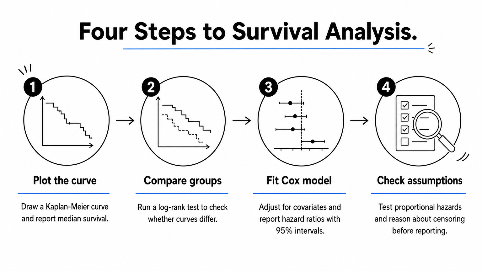
- Plot a Kaplan-Meier curve and report median survival and the number at risk.
- Compare groups with a log-rank test.
- Fit a Cox model with your covariates and report hazard ratios with 95% confidence intervals.
- Check the assumptions before you trust any of it.
Run it in code or in a workspace
In Python, the lifelines library covers steps 1 and 3. In R, the survival package does the same with survfit and coxph.
from lifelines import KaplanMeierFitter, CoxPHFitter

kmf = KaplanMeierFitter()
kmf.fit(durations=df["months"], event_observed=df["event"])
kmf.plot_survival_function()

# df should contain only the time, event, and numeric covariate columns
cph = CoxPHFitter()
cph.fit(df, duration_col="months", event_col="event")
cph.print_summary()
In PlotStudio, you upload the dataset and ask for Kaplan-Meier curves by treatment and a Cox model in plain English. Verification Mode lets you review and edit the plan before it runs, and you can inspect the generated Python afterward. The choice of method stays yours.
Define the event and the time zero first, because no model can fix a vague clock.
Survival analysis models and when each one fits
The main survival analysis models are Kaplan-Meier, the log-rank test, Cox proportional hazards, parametric models, and competing risks methods. You choose among them by the question you ask, not by which sounds most advanced.
Survival and hazard: the two ideas behind every model
The survival function, S(t), is the probability that a subject survives beyond time t. It starts at 1 and only falls. The hazard function, h(t), is the instantaneous event rate at time t among those still event-free. Survival is cumulative, while hazard describes the current risk.
Comparing the main models
| Model | Question it answers | Main output | Key condition |
|---|---|---|---|
| Kaplan-Meier | How does survival change over time? | Survival curve, median survival | Right-censored data, no covariates |
| Log-rank test | Do two or more groups differ? | p-value | Works best when curves do not cross |
| Cox proportional hazards | Which variables affect the event rate? | Hazard ratios | Proportional hazards |
| Parametric (Weibull, exponential, log-normal) | What survival curve fits, and what happens beyond follow-up? | Fitted distribution, predictions | A correctly chosen distribution |
| Competing risks (cumulative incidence, Fine-Gray) | What happens when another event blocks the one of interest? | Cumulative incidence per event | Defined competing events |
Cox regression is the default when you need adjusted effects. A hazard ratio of 0.70 means the event rate is 30% lower in one group than in the other at any given time. Choose a parametric model when you must extrapolate beyond your follow-up, and accept that a wrong distribution gives wrong forecasts.
Pick the model that matches your question: curves describe, tests compare, and Cox regression adjusts.
Worked example: a Kaplan-Meier curve by hand
A Kaplan-Meier estimate multiplies, at each event time, the fraction of at-risk subjects who survive that moment. Here is a small dataset of 10 patients followed in months. Events occurred at 3, 5, 8, 8, 12, and 15. Patients were censored at 6, 10, 18, and 20.
The calculation
| Time (months) | At risk | Events | Censored | Survival S(t) |
|---|---|---|---|---|
| 3 | 10 | 1 | 0 | 0.900 |
| 5 | 9 | 1 | 0 | 0.800 |
| 6 | 8 | 0 | 1 | 0.800 |
| 8 | 7 | 2 | 0 | 0.571 |
| 10 | 5 | 0 | 1 | 0.571 |
| 12 | 4 | 1 | 0 | 0.429 |
| 15 | 3 | 1 | 0 | 0.286 |
At month 3, one of 10 patients has the event, so S = 9/10 = 0.900. At month 5, S = 0.900 × 8/9 = 0.800. At month 8, two of the 7 at risk have events, so S = 0.800 × 5/7 = 0.571. At month 12, S = 0.571 × 3/4 = 0.429. At month 15, S = 0.429 × 2/3 = 0.286.
Reading the result
Notice what censoring did. At months 6 and 10, the curve did not move, but the number at risk shrank, so later events weighed more heavily. That is how a censored patient contributes information without being counted as an event.

The median survival is 12 months, the first time the curve drops to 0.50 or below. The curve reaches 0.429 at month 12, so that is where it crosses. If you treated the four censored patients as events, you would report a far shorter median.
A censored patient never moves the curve down, but still shapes every estimate after their last visit.
Assumptions and mistakes that break survival data analysis
Survival methods are only as trustworthy as their assumptions, and the two that matter most are non-informative censoring and proportional hazards. Check both before you report any result.
The assumptions to check
Non-informative censoring means subjects who are censored have the same future risk as comparable subjects who stay in the study. If sicker patients drop out early, your curve looks better than reality. You cannot test this with the data alone, so you have to reason about why people were censored.
Proportional hazards means the hazard ratio between groups stays constant over time. Crossing Kaplan-Meier curves are a clear warning sign. A formal check uses scaled Schoenfeld residuals. If the assumption fails, consider stratifying the model, adding time-dependent terms, or reporting results by time period.
Mistakes that appear in real papers
- Treating censored cases as events or deleting them, which biases the curve.
- Ignoring competing events. If death prevents relapse, treating death as ordinary censoring can overstate relapse incidence.
- Too few events. A common rule of thumb is about 10 events per predictor in a Cox model, and it counts events, not patients.
- Over-reading the tail. When only a handful of subjects remain at risk, the end of the curve is unstable.
- Vague time zero. Mixing start points, such as diagnosis for some and treatment start for others, makes the times incomparable.
Report the number at risk under every curve, so readers can judge how far to trust the tail.
Putting survival analysis to work
Survival analysis is the right tool whenever your outcome is the time until an event and some cases are still unfinished. Define the event and the start of the clock, code each subject as event or censored, describe survival with Kaplan-Meier, compare groups with the log-rank test, and adjust with Cox regression. Then check censoring and proportional hazards before you publish a number.
Once you understand these steps, the software part is the easy bit. If you want to run them on your own dataset and see the code behind every result, you can run Kaplan-Meier and Cox analyses in PlotStudio AI and review the methods before they execute.