Survival Analysis Basics: A Beginner’s Guide to Time-to-Event Data

Survival analysis models the time until a defined event occurs and handles observations that never reach that event, a problem statisticians call censoring. It is a set of statistical procedures for analyzing time-to-event data, not just death rates, and its scope covers any binary outcome: relapse, machine failure, remission, or customer churn, as NCBI’s StatPearls primer makes clear. Censoring matters because incomplete follow-up is the rule, not the exception, in almost every real dataset.
The core beginner toolkit has three parts, and this guide walks through each one in order:
- Kaplan-Meier estimator: builds the survival curve and estimates median survival time
- Log-rank test: compares survival curves between two or more groups
- Cox proportional hazards model: quantifies how covariates change the hazard, adjusting for multiple variables at once
Key Takeaways
Survival analysis works because it treats incomplete follow-up as information rather than a flaw, using Kaplan-Meier, the log-rank test, and Cox regression to extract valid conclusions from censored time-to-event data.
| Point | Details |
|---|---|
| Censoring is not missing data | Right, left, and interval censoring must be coded and retained, never dropped, to avoid biased estimates. |
| Kaplan-Meier is descriptive first | Use it to visualize survival and report median time, confidence intervals, and the number at risk. |
| Log-rank tests compare, Cox quantifies | Log-rank gives a p-value for group differences; Cox gives adjusted hazard ratios with confidence intervals. |
| Check assumptions before trusting output | Proportional hazards and non-informative censoring both need verification, not assumption. |
| Reproducibility tools reduce analytic error | Plotstudio’s pre-approved analysis plans and local execution help lock in consistent time-origin and variable definitions for peer-reviewed work. |
Table of Contents
- Understanding Censoring: Right, Left, and Interval Types
- How Do Kaplan-Meier Survival Curves Work?
- What Does the Log-Rank Test Actually Compare?
- Cox Proportional Hazards: Reading Hazard Ratios Correctly
- When Should You Use KM Versus Cox Regression?
- How Do You Run a Basic Survival Analysis Workflow?
- Building Reproducible Survival Analysis for Peer Review
- What Is a Survival Function Versus a Hazard Function?
- What Are Parametric Survival Models Like Weibull and Exponential?
- How Much Data Do You Need for Survival Analysis?
- The Gap Between Teaching Survival Analysis and Doing It Right
- Turn Your Survival Data Into a Reproducible Analysis
- Frequently Asked Questions About Survival Analysis Basics
- Sources
Understanding Censoring: Right, Left, and Interval Types
Censoring happens when you know a subject’s follow-up time but not whether or exactly when the event occurred. Right-censoring is the most common form: a patient is still alive when the study ends, or a customer is still subscribed when the data pull happens. You know they haven’t hit the event yet, but you don’t know when they will. Left-censoring is rarer and trickier. It occurs when the event already happened before observation started. Think of a study screening for a disease’s onset where some participants were already infected before enrollment. You know the event occurred, just not exactly when. Interval-censoring sits between the two. The event happened somewhere between two check-ins, such as a tumor recurrence detected only at a quarterly scan.
Throwing out censored cases is one of the most common mistakes new analysts make. It biases results toward the subjects who experienced the event fastest, since long survivors are disproportionately the ones still enrolled and therefore excluded. PMC’s clinician primer is direct on this point: survival methods incorporate incomplete observations rather than discarding them, which is precisely what makes Kaplan-Meier and Cox regression different from ordinary regression tools.
Here’s how a single right-censored case gets recorded in a dataset:
- Patient enrolls on day 0 with time origin set at diagnosis.
- Study ends on day 730 with no relapse observed.
- The record shows: time = 730, event = 0 (censored), covariates as measured at baseline.
Pro Tip: Always code your censoring indicator explicitly (1 = event, 0 = censored) in a dedicated column, and double check it against your event-date field before running anything. A silent coding error here quietly corrupts every downstream estimate.
How Do Kaplan-Meier Survival Curves Work?
A Kaplan-Meier curve starts at 1.0, meaning 100% of the group is event-free at time zero, and steps downward each time an event occurs. It never rises, and censoring doesn’t cause a drop. Censored subjects simply leave the risk set at their last known follow-up point without pulling the curve down. This stepwise shape is what separates Kaplan-Meier from a smooth theoretical curve. It is a nonparametric estimator, meaning it makes no assumption about the underlying distribution of survival times, which is exactly why it’s the default starting point for describing time-to-event data, according to PMC’s basic concepts review.
Reading a KM curve well means looking past the shape and checking the numbers underneath it.
- Median survival: the time point where the curve crosses 0.5, meaning half the group has experienced the event.
- Confidence intervals: shown as a shaded band or bracket around the curve; wide bands late in follow-up usually signal a shrinking risk set, not necessarily more uncertainty about the treatment effect.
- Number at risk table: placed beneath the plot, this shows how many subjects remain under observation at each time point, which tells you how much to trust the tail of the curve.
- Curve separation: two curves that visibly diverge and stay apart suggest a survival difference between groups worth testing formally.
The KM curve can start at 1.0 and end well above zero if the study period ends before most subjects experience the event, which is normal in cancer trials with short follow-up. Kaplan-Meier is the right descriptive tool whenever you want to summarize survival for one group or eyeball a difference between a small number of groups, before or instead of building a regression model. It answers “what does survival look like,” not “why does it look that way,” which is where the log-rank test and Cox regression take over.
What Does the Log-Rank Test Actually Compare?
The log-rank test asks a specific question: do two or more Kaplan-Meier curves differ across the entire follow-up period? The null hypothesis states there is no difference in survival between groups at any time point. A small p-value (conventionally below 0.05) means the observed separation between curves is unlikely under that null, so you reject it and conclude the groups differ.
The test carries assumptions that beginners routinely skip past:
- Censoring must be non-informative, meaning the reason a subject drops out is unrelated to their underlying risk of the event.
- Groups should have comparable entry patterns and follow-up structure, not systematically different enrollment timing.
- The test performs best when hazards between groups stay roughly proportional over time; curves that cross are a warning sign.
The log-rank test’s biggest limitation is that it gives you a p-value, not an effect size. It tells you groups differ, not by how much or in which direction, adjusted for anything else. When curves cross or hazards clearly shift over time, weighted variants like the Wilcoxon or Tarone-Ware tests, or a Cox model with time-dependent terms, handle the comparison better.
Cox Proportional Hazards: Reading Hazard Ratios Correctly
The Cox model is semi-parametric: it estimates how covariates affect the hazard rate while leaving the baseline hazard function completely unspecified. That flexibility is why it dominates multivariable survival modeling. You don’t need to guess the shape of the underlying hazard, only how covariates shift it relative to each other, per PMC’s Cox regression overview.
The output you’ll report is the hazard ratio (HR), typically with a 95% confidence interval. An HR of 1.8 for a treatment variable means the hazard, the instantaneous risk of the event, is 80% higher in that group at any given moment, holding other covariates constant. An HR below 1.0 signals a protective effect; an HR of exactly 1.0 means no association. If the 95% CI crosses 1.0, the effect isn’t statistically distinguishable from no effect at your chosen threshold.
Reading Cox output responsibly means checking a few things before trusting the hazard ratio:
- Verify the proportional hazards assumption, typically with Schoenfeld residuals, since Cox assumes the hazard ratio between groups stays constant over the entire follow-up period.
- Watch for time-dependent effects. A treatment that helps early but not late will violate proportional hazards and needs a time-varying covariate term.
- Check for adequate events per covariate. Too many predictors relative to the number of events produces unstable estimates.
Pro Tip: Don’t treat Cox regression as the default choice just because it handles multiple covariates. Freedman’s primer on survival analysis warns that Cox models are frequently applied where simpler methods would suffice, resting on proportional hazards assumptions that are rarely checked and often unjustified in practice.
When Should You Use KM Versus Cox Regression?
The decision usually comes down to one question: do you need to adjust for covariates, or are you just comparing groups? Kaplan-Meier with a log-rank test is the right call for a simple, unadjusted comparison of two or three groups where you want a visual and a p-value, nothing more. Cox regression becomes necessary the moment you need an adjusted hazard ratio, multiple predictors, or continuous covariates in the model.
Run through this checklist before choosing a method:
- Sample size and event count: fewer than roughly 10 events per covariate makes Cox unstable; lean on KM and log-rank instead.
- Censoring proportion: heavy censoring (over 50%) demands closer scrutiny of whether it’s informative before trusting either method.
- Need for adjustment: if confounders exist (age, disease stage, baseline severity), Cox is the only option among the two that handles them.
- Time-dependent covariates: if a predictor changes value during follow-up (a lab value measured repeatedly), a time-varying Cox extension is required, not a static model.
| Scenario | Recommended method |
|---|---|
| Comparing two treatment arms, no confounders | Kaplan-Meier plus log-rank test |
| Estimating adjusted risk across several predictors | Cox proportional hazards model |
| Predictor value changes during follow-up | Cox with time-dependent covariates |
| Multiple event types competing (e.g., death vs. relapse) | Competing risks framework (Fine-Gray or cause-specific hazards) |
That last row deserves its own caution. When subjects can experience one of several distinct event types, and experiencing one removes them from risk of the others, standard KM and Cox methods can overstate risk. Competing risks models are a separate topic worth consulting a biostatistician about before applying casually.
How Do You Run a Basic Survival Analysis Workflow?
Before writing any code, get the data structure right. Every survival dataset needs a consistent time origin (diagnosis date, enrollment date, treatment start), a clearly coded event indicator, a censoring flag, and any covariates you plan to adjust for.
The sequence that works for almost every first analysis:
- Plot a Kaplan-Meier curve for the overall sample and by key subgroups to see the shape of survival.
- Run a log-rank test if you’re comparing two or more groups without needing adjustment.
- Fit a Cox model if you need adjusted hazard ratios or have continuous covariates.
- Check the proportional hazards assumption on the Cox model before reporting anything.
For software, the choice is straightforward. In R, the survival package covers KM, log-rank, and Cox in one consistent framework, and its vignettes on CRAN walk through time-dependent covariates in detail. In Python, lifelines and scikit-survival provide equivalent functionality with a more object-oriented syntax.
Whatever tool you use, your final write-up should report:
- Hazard ratios with 95% confidence intervals for every covariate in the Cox model
- P-values from the log-rank test, clearly labeled as comparing curves, not estimating effect size
- Median survival time with its confidence interval, and the number at risk at key follow-up points
- Results of the proportional hazards assumption check
Building Reproducible Survival Analysis for Peer Review
Reviewers increasingly expect a documented time-origin definition and a pre-specified analysis plan, not results assembled after the fact. Platforms like Plotstudio gate each analysis behind a plan the researcher approves before code runs, which keeps variable definitions and thresholds fixed from the start. Local execution matters too: data governed by IRB or GDPR rules never has to leave the researcher’s machine.
- Pre-approved plans lock in time origin, event coding, and covariate specification.
- Local processing supports patient-level data under IRB or GDPR restrictions.
- Exportable notebooks and PDF reports give reviewers a traceable audit trail.
What Is a Survival Function Versus a Hazard Function?
The survival function, written S(t), gives the probability that a subject survives past time t without experiencing the event. It’s what a Kaplan-Meier curve plots directly: at t=0, S(t)=1, and it decreases monotonically as time passes.
The hazard function, h(t), is different in kind, not just in name. It represents the instantaneous risk of the event occurring at time t, given that the subject has survived up to that point. Think of it as a rate, not a probability: a hazard of 0.05 per month doesn’t mean a 5% chance over the whole study, it means an instantaneous risk that compounds continuously. Hazard functions can rise, fall, or stay flat over time, and their shape reveals whether risk accelerates (as with mechanical wear-out) or declines (as with post-surgical recovery).
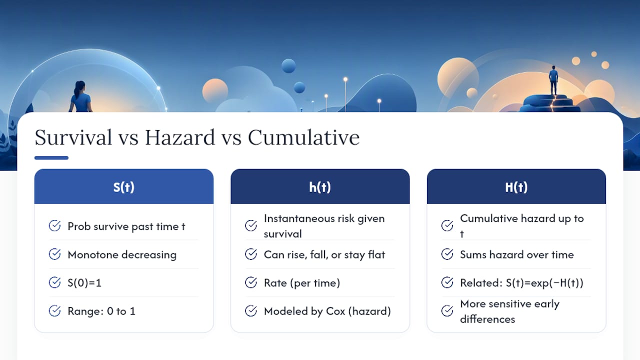
The cumulative hazard function, H(t), sums the hazard up to time t and connects mathematically to the survival function through the relationship S(t) = exp(negative H(t)). Analysts sometimes prefer plotting cumulative hazard instead of survival probability because it’s more sensitive to small changes early in follow-up, making differences between groups easier to spot visually before they show up clearly on a KM curve.
Understanding these three functions matters because Cox regression models the hazard function directly, not the survival function. That’s why the model’s output is a hazard ratio rather than a difference in survival probability. A researcher who only understands S(t) will misread what a Cox coefficient is actually telling them.
What Are Parametric Survival Models Like Weibull and Exponential?
Kaplan-Meier and Cox regression are both largely distribution-free, but parametric survival models take a different approach: they assume survival times follow a specific probability distribution, and they estimate the parameters of that distribution directly from data.
The exponential model is the simplest case. It assumes a constant hazard over time, meaning the risk of the event doesn’t change whether a subject has been at risk for one day or one year. That assumption fits few real biological processes, but it’s useful as a baseline or for early-stage reliability testing where failure is genuinely random over time.
The Weibull model relaxes that constraint by adding a shape parameter that lets the hazard increase, decrease, or stay flat over time. A shape parameter above 1 signals increasing risk, common in aging or wear-out processes; below 1 signals decreasing risk, typical of early mechanical failures or post-treatment recovery periods.
Parametric models offer two practical advantages over Kaplan-Meier. First, they extrapolate: if your follow-up ends before most events occur, a fitted Weibull curve can project survival beyond the observed data, something Kaplan-Meier cannot do responsibly. Second, they’re more efficient with small samples, since they borrow strength from the assumed distribution rather than estimating each point empirically.
The tradeoff is real, though. If the chosen distribution doesn’t match the true underlying process, parametric estimates can be systematically wrong in ways a nonparametric Kaplan-Meier curve never would be. Beginners should treat parametric models as a second step after visualizing Kaplan-Meier curves, not a replacement for them.
How Much Data Do You Need for Survival Analysis?
Sample size in survival analysis hinges less on the total number of subjects and more on the number of events observed, which surprises most people coming from standard regression backgrounds. A dataset with 5,000 subjects but only 40 deaths has far less statistical power than a dataset with 500 subjects and 200 events.
For Cox regression specifically, a widely used rule of thumb calls for at least 10 events per covariate to keep hazard ratio estimates stable. A model with five predictors, then, ideally needs 50 or more observed events, not 50 total subjects. Fall short of that, and standard errors inflate, confidence intervals widen unhelpfully, and the model risks overfitting to noise in the data.

Censoring proportion complicates this further. Before collecting data, it helps to estimate the expected event rate from prior literature or pilot data and work backward to the enrollment target needed to hit your event count, rather than picking a sample size based on total subjects alone.
For log-rank test comparisons between two groups, power depends heavily on the anticipated hazard ratio between them. Detecting a modest survival difference (say, an HR of 1.3) requires substantially more events than detecting a large one (an HR of 3.0). Underpowered survival studies are common in practice, and a non-significant log-rank result from a low-event study should never be read as proof of “no difference.”
The Gap Between Teaching Survival Analysis and Doing It Right
Most introductions to survival analysis treat Kaplan-Meier, log-rank, and Cox regression as a fixed sequence: plot the curve, test the groups, fit the model, report the hazard ratio. That sequence isn’t wrong, but it skips the part that actually determines whether the results hold up: whether the analyst checked assumptions before trusting output, and whether the time origin, event coding, and covariate choices were locked in before anyone saw the results.
The conventional advice undersells how often Cox models get misapplied to datasets where proportional hazards clearly doesn’t hold, or where informative censoring quietly invalidates the whole exercise. Freedman’s warning about analysts reaching for Cox by default, rather than checking whether the assumptions fit, deserves more attention than it gets in most beginner tutorials.
If there’s one thing a new analyst should prioritize, it’s discipline over sophistication: define your time origin and event coding before you touch the data, plot Kaplan-Meier before fitting anything multivariable, and treat assumption checks as mandatory steps, not optional afterthoughts. The method matters less than the rigor you bring to applying it.
Turn Your Survival Data Into a Reproducible Analysis
If you’ve followed this guide this far, you already know that the hardest part of survival analysis usually isn’t the math. It’s making sure your time-origin definition, censoring codes, and assumption checks stay consistent from the first Kaplan-Meier plot through the final Cox model, especially when a reviewer asks you to reproduce it six months later. Plotstudio builds that discipline into the workflow itself: every analysis runs behind an analysis plan you approve up front, so your methods and thresholds are locked in before any code executes, functioning as a built-in audit trail for your methods section.

Because analysis runs locally on your own machine, patient-level data governed by IRB or GDPR rules never has to leave your device, a real constraint for clinical researchers that most cloud-based tools simply can’t satisfy. Plotstudio runs both R and Python natively and covers Cox proportional hazards alongside the mixed-effects models and regression work that typically accompanies survival analysis in a full research paper, then exports annotated notebooks and PDF reports a supervisor or reviewer can trace line by line. If you’re preparing a thesis chapter, a grant application, or a peer-reviewed manuscript, explore Plotstudio’s platform and see how a pre-specified analysis plan can tighten your next survival analysis before you write a single line of code.
Frequently Asked Questions About Survival Analysis Basics
What is the simplest way to explain survival analysis basics to a beginner? Survival analysis basics come down to modeling how long it takes for an event to happen and accounting for subjects who haven’t experienced it yet by the time the study ends. Kaplan-Meier, the log-rank test, and Cox regression form the essential starting toolkit.
Do I need Cox regression if I only have two groups to compare? Not necessarily. If you don’t need to adjust for covariates, a Kaplan-Meier curve with a log-rank test answers the comparison question directly and avoids the proportional hazards assumption Cox requires.
What’s the difference between a survival curve and a hazard curve? A survival curve shows the probability of remaining event-free over time, always starting at 1.0 and decreasing. A hazard curve shows the instantaneous risk of the event at each moment, which can rise, fall, or stay flat depending on the underlying process.
How many events do I need before running a Cox model? A common guideline calls for at least 10 observed events per covariate in the model. Fewer events than that produces unstable hazard ratio estimates with wide confidence intervals.
Can I ignore censored observations if there aren’t very many? No. Even a small proportion of censored cases can bias results if excluded, because the subjects still enrolled at study end tend to be systematically different from those who already experienced the event. Survival methods are built specifically to include them correctly.
Sources
- Survival Analysis - StatPearls - NCBI Bookshelf
- Survival analysis: A primer for the clinician scientists - PMC
- Survival analysis: A primer (Freedman) - UC Berkeley