Time Series Forecasting for Data Scientists: Methods and Workflows

Time series forecasting predicts future values by modeling patterns in historical, time-stamped data. It works by isolating trend, seasonality, and noise from past observations, then projecting how those patterns are likely to continue. Analysts and researchers use it to improve planning, allocate resources before demand shifts, and flag anomalies before they become costly.
The technique underpins decisions with a clear time horizon and a measurable cost of being wrong. A hospital forecasting bed occupancy, a lab projecting reagent consumption, and a finance team modeling quarterly revenue are all solving the same structural problem with different data.
- Who it serves: data scientists building production pipelines, analysts supporting operational decisions, researchers who need defensible, reproducible projections for publication
- Typical horizons: short-term (days to weeks) for operational decisions, medium-term (months) for budgeting, long-term (years) for capacity and infrastructure planning
- Core requirement: enough historical observations, at a consistent frequency, to separate real signal from random variation
Key Takeaways
Accurate time series forecasting depends less on model sophistication than on correct stationarity diagnosis, honest rolling-origin validation, and a documented audit trail from raw data to final forecast.
| Point | Details |
|---|---|
| Diagnose before modeling | Run ADF and KPSS tests together, since they can disagree and reveal trend stationarity that either test alone would miss. |
| Match model to constraints | Choose classical, ML, or deep learning based on data size, interpretability needs, and compute budget, not benchmark hype. |
| Validate with rolling origin | Standard k-fold cross-validation leaks future data into training and inflates accuracy scores for temporal data. |
| Report probabilistic, not just point, forecasts | Use CRPS and calibration checks to confirm your prediction intervals hold their stated coverage. |
| Document every run for reproducibility | Plotstudio’s plan-approval workflow and local execution give researchers an auditable, privacy-preserving path from raw series to published forecast. |
Table of Contents
- What Is Time Series Forecasting and What Are Its Core Components?
- When Should You Use Time Series Forecasting?
- How Do You Prepare Data for Reliable Forecasting?
- How Do You Detect Stationarity and Seasonality?
- Which Forecasting Model Family Should You Choose?
- How Do You Train, Validate, and Evaluate a Forecasting Model?
- How Do You Build an End-to-End Forecasting Pipeline?
- What Tools and Libraries Do Researchers Actually Use?
- How Does PlotStudio Support Research-Grade Forecasting?
- The Overrated Metric and the Underrated Discipline
- Turn Forecasting Diagnostics Into Reproducible Results
- Where to Go Deeper on Time Series Forecasting
- Sources
What Is Time Series Forecasting and What Are Its Core Components?
Forecasting, at its core, means estimating how a sequence of observations will continue given what it has already done. That sounds simple until you try to define “continue” precisely. A point forecast gives you a single expected value. A probabilistic forecast gives you a distribution, or at minimum a prediction interval, which is almost always the more honest answer when you’re reporting results in a paper or a grant application. Forecasting: Principles and Practice draws this distinction early because it shapes every downstream modeling choice, including which loss function you optimize and how you communicate uncertainty to a reader who isn’t a statistician.
Every time series decomposes into a handful of structural pieces:
- Trend: the long-run direction, upward, downward, or flat, once short-term noise is smoothed away
- Seasonality: a pattern that repeats at a fixed, known frequency, like daily traffic cycles or quarterly retail spikes
- Cycle: a fluctuation without a fixed period, often tied to economic or biological cycles longer than a calendar year
- Level: the baseline value the series would sit at absent trend or seasonal effects
- Noise: the irreducible randomness left after you’ve accounted for everything else
- Autocorrelation: the degree to which a value depends on its own past values, the property that separates time series models from standard regression
That autocorrelation structure is the whole reason time series methods exist as a separate discipline. Cross-sectional models assume independent observations; a time series violates that assumption by design, which is why standard regression diagnostics don’t transfer cleanly.
A statistic worth internalizing: reliable pattern detection generally needs a substantial number of observations, because with too few data points, a discovered “trend” or “seasonal pattern” is often indistinguishable from a chance fluctuation. Before you commit to a model family, plot the raw series, then a seasonal subseries plot, then the autocorrelation function (ACF) and partial autocorrelation function (PACF). Skipping this step is the single most common reason a forecasting project produces a model that looks fine in validation and falls apart in production.
When Should You Use Time Series Forecasting?
Forecasting earns its place when you have a repeatable measurement, taken over time, feeding a decision with a real cost of error. It’s the wrong tool when you’re trying to establish why something happened rather than predict what happens next.
Common, well-matched use cases include:
- Demand forecasting: inventory and staffing decisions where overordering and stockouts both carry a quantifiable cost
- Capacity planning: server load, hospital bed occupancy, or manufacturing throughput, where lead times for scaling capacity are long
- Financial forecasting: revenue, cash flow, and risk exposure projections tied to reporting cycles
- Energy load forecasting: grid operators balancing generation against predicted consumption in near real time
- Experiment and clinical monitoring: tracking a metric over the course of a trial to catch drift or adverse trends early
The horizon you need should match the lead time of the decision it informs. A staffing decision made two days out needs a short-term forecast with tight intervals; a facility expansion decision made three years out can tolerate wider uncertainty because you have time to course-correct. Matching horizon to actionability, rather than forecasting as far as the data will technically allow, is what separates useful forecasts from decorative ones.
Forecasting is the wrong tool when the real question is causal: does a marketing campaign cause a sales lift, or did it just coincide with one? For that, you want a controlled experiment or a causal inference design, not an extrapolation of past patterns. Treating correlation-driven forecasts as if they answer causal questions is a common and expensive mistake in applied research.
How Do You Prepare Data for Reliable Forecasting?
Preprocessing quality determines forecast quality more reliably than model choice does. A well-tuned ARIMA model on a poorly cleaned series will underperform a naive baseline on a well-prepared one.
- Check volume and frequency first. There’s no universal minimum, but a rule of thumb for seasonal models is at least two to three full seasonal cycles of history, so a monthly series with annual seasonality needs two to three years of data at minimum. GeeksforGeeks’ overview of forecasting workflows lists this alongside the standard preprocessing steps most practitioners reach for first.
- Resolve missing timestamps and irregular sampling. Resample to a consistent frequency (hourly, daily, monthly) before doing anything else. Linear interpolation works for short gaps; for longer gaps, consider seasonal interpolation or explicit missingness flags rather than silently filling values.
- Handle outliers deliberately, not automatically. A demand spike from a real promotional event is signal, not noise, so removing it blindly will bias your seasonal estimates. Winsorizing or capping is safer than deletion when you’re unsure.
- Apply transformations to stabilize variance. A log transform or Box-Cox transformation tames series where variance grows with the level, which is common in financial and retail data and violates the constant-variance assumption most classical models need.
- Scale features for ML and deep learning models. Statistical models like ARIMA don’t require scaling, but tree ensembles and neural networks generally converge faster and perform better on normalized inputs.
- Engineer lags, rolling statistics, and calendar features. Lagged values, rolling means and standard deviations, day-of-week and holiday indicators, and external regressors like price or weather all give ML models the temporal context that classical models get for free from their structure.
Pro Tip: Don’t interpolate across a structural break, like a supply chain disruption or a policy change, as if it were a normal gap. Split the series at the break point and treat the segments separately, or your model will learn a blended pattern that describes neither period accurately.
Outlier handling deserves its own attention beyond the basic checklist above; a deeper look at outlier detection methods covers approaches suited specifically to sequential data, where a value can be anomalous relative to its neighbors even if it looks unremarkable in the overall distribution.
How Do You Detect Stationarity and Seasonality?
A stationary series has a constant mean, variance, and autocorrelation structure over time, and most classical forecasting models either assume it or require you to transform your way to it. Two tests dominate practice: the Augmented Dickey-Fuller (ADF) test, which checks for a unit root under the null hypothesis of non-stationarity, and the KPSS test, which flips that null to test for stationarity directly. Running both is standard practice, because they can disagree, and a disagreement usually tells you the series is trend-stationary rather than cleanly stationary or non-stationary. When either test signals a problem, differencing (subtracting each value from its predecessor) or detrending usually resolves it.
Seasonality detection starts visually. A seasonal subseries plot, where you overlay each cycle on top of the others, will often show the pattern before any statistic confirms it. The ACF and PACF plots back that up: a strong spike at lag 12 in monthly data is a clear annual seasonality signal. Fourier analysis is the more rigorous option when you suspect multiple overlapping seasonal periods, since it decomposes the series into constituent frequencies rather than testing for one period at a time.
A statistic worth internalizing: automated seasonality detection is now a standard feature in production libraries, not a manual, one-off analysis step. Microsoft’s ML.NET, for example, ships a DetectSeasonality API that returns a detected seasonal period or -1 if none is found, and it accepts a configurable randomness threshold so you can tune how confident the algorithm needs to be before it commits to a seasonal call. That threshold matters enormously at scale: run automated detection across a few thousand SKUs and a loose threshold will hallucinate seasonality in pure noise.
- Multiple seasonalities (daily and weekly, or weekly and annual) require models built to handle them explicitly, like TBATS or Fourier-term regression, rather than a single seasonal ARIMA
- Choosing the wrong seasonal period is a common silent failure; if your ACF spike doesn’t line up with a plausible real-world cycle, question the detection before trusting it
- For trading calendars and holiday-driven gaps specifically, BacktestMarket’s guide to handling holiday gaps in market data walks through the recurring calendar effects that standard seasonal decomposition tends to miss
Which Forecasting Model Family Should You Choose?
There’s no single best model family. There’s a best model for your data size, your stationarity profile, your interpretability requirements, and your compute budget, and those constraints usually narrow the field faster than any accuracy benchmark does.
Classical statistical models
Naive baselines, persistence forecasts, and seasonal naive methods should be your first stop, not an afterthought. If a sophisticated model can’t beat “tomorrow will look like today, adjusted for last year’s seasonal pattern,” the sophisticated model isn’t earning its complexity. Exponential smoothing methods, especially the Holt-Winters variant, handle trend and seasonality directly through weighted averages that decay exponentially into the past, and they remain remarkably competitive on short, clean series. ARIMA models (AutoRegressive Integrated Moving Average) generalize further, combining autoregression, differencing, and moving-average error correction into one framework. Forecasting: Principles and Practice treats ARIMA and exponential smoothing as complementary rather than competing, since they’re built on different theoretical assumptions and often win on different series within the same dataset.
Classical models assume linearity and a clear, extractable seasonal structure. They’re data-efficient, need relatively little history to fit well, and produce coefficients you can defend in a peer review. Their weakness shows up when relationships are nonlinear or when you have dozens of interacting external regressors, which is exactly where the next family takes over.
Machine learning models with covariates
Tree ensembles like gradient boosted trees, and regularized regressions, can incorporate lags, rolling statistics, and exogenous variables as ordinary features, sidestepping the strict distributional assumptions classical models need. They tend to help when you have rich external data, price, weather, promotional calendars, that plausibly drives the outcome, and when the relationship between those drivers and the target is nonlinear.

The pitfall is subtle and common: standard cross-validation shuffles data randomly, which leaks future information into training folds and produces a validation score that collapses in production. Any ML model applied to time series data needs validation that respects temporal order, a point worth internalizing before you touch the metrics section below.
Deep sequence models and transformers
Long Short-Term Memory (LSTM) and Gated Recurrent Unit (GRU) networks were the first deep architectures to handle sequential dependencies without hand-engineered lag features, and they still perform well on multivariate series with long memory requirements. More recent architectures, the Temporal Fusion Transformer, N-BEATS, and N-HiTS, have pushed further, and benchmark work through projects like sktime and PyTorch Forecasting shows these newer architectures often outperform older baselines on large-scale univariate forecasting competitions. That advantage tends to show up specifically when you have many related series to train on jointly and long prediction horizons where classical models compound error quickly.
Deep models are data-hungry and computationally expensive relative to a Holt-Winters fit that runs in milliseconds. If you have thirty related series and a laptop, a transformer is probably overkill. If you have thirty thousand SKUs and a GPU cluster, it may be the only approach that scales.
Pro Tip: Before reaching for a deep model, fit a seasonal naive baseline and an ARIMA model on the same data and log both scores. If your final model can’t beat the naive baseline by a meaningful margin, the added complexity isn’t buying you anything, and a reviewer will ask exactly that question.
| Consideration | Favors classical (ARIMA/ETS) | Favors ML with covariates | Favors deep learning/transformers |
|---|---|---|---|
| Data size | Short series, single series | Moderate history, rich covariates | Many related series, long history |
| Interpretability need | High (coefficients, confidence intervals) | Moderate (feature importance) | Low to moderate |
| Compute budget | Minimal | Moderate | High |
| Probabilistic forecasts needed | Built-in for ETS/ARIMA | Requires additional quantile modeling | Native in some architectures (DeepAR, TFT) |
How Do You Train, Validate, and Evaluate a Forecasting Model?
Standard k-fold cross-validation is invalid for time series because it trains on future data to predict the past, a look-ahead error that inflates your validation score and evaporates in production. The correct approach is rolling-origin or expanding-window cross-validation: train on an initial window, forecast the next block, then slide the origin forward and repeat. This gives you multiple, temporally honest estimates of how the model performs at the horizon you actually care about, not just one lucky or unlucky split.
- Choose your evaluation horizon deliberately. A model tuned for one-step-ahead accuracy can perform very differently at a twelve-step horizon, so evaluate at every horizon you plan to deploy against.
- Select metrics that match your reporting need. Mean Absolute Error (MAE) is robust to outliers and easy to explain to non-technical stakeholders. Root Mean Squared Error (RMSE) penalizes large errors more heavily, which matters when big misses are disproportionately costly. Mean Absolute Percentage Error (MAPE) gives you a scale-free number for comparing across series, but it breaks down near zero values, so check your data before defaulting to it.
- Evaluate probabilistic forecasts separately from point forecasts. The Continuous Ranked Probability Score (CRPS) scores an entire predicted distribution against the observed outcome, and calibration checks confirm that your 90% prediction interval actually contains the true value roughly 90% of the time.
- Audit for leakage before trusting any result. Check that no feature used at training time, a rolling average that accidentally includes the target period, a scaler fit on the full dataset, could only be known after the forecast date.
- Log every run for reproducibility. Model version, training window, hyperparameters, and random seed all need to be recoverable months later when a reviewer or collaborator asks how a specific number was produced.
Pro Tip: Track forecast error against a rolling baseline over time, not just at deployment. A model that degrades slowly as the underlying process shifts, a classic case of concept drift, won’t trigger an obvious failure; it’ll just quietly get worse until someone notices the decisions built on it were wrong for months.
Monitoring in production means setting alert thresholds on error metrics and retraining on a fixed cadence or when drift crosses a defined bound, rather than retraining reactively after a visible failure. A deeper look at validation and estimation techniques for forecasting accuracy covers the identification and estimation steps that precede this validation stage in more detail.
How Do You Build an End-to-End Forecasting Pipeline?
A forecasting project moves through the same stages regardless of which model family you end up choosing, and skipping a stage is where most production failures originate.
- Ingest the raw data and confirm its frequency, time zone, and any known collection gaps.
- Explore with run charts, seasonal subseries plots, and ACF/PACF diagnostics before writing a single line of modeling code.
- Preprocess by resampling to a consistent frequency, handling missing values, and applying variance-stabilizing transforms.
- Engineer features, including lags, rolling statistics, calendar indicators, and any exogenous regressors you have reliable future values for.
- Select and fit models, starting with a naive baseline and moving up in complexity only as each step earns its keep.
- Validate using rolling-origin cross-validation at every horizon you plan to deploy against.
- Deploy the chosen model with logged configuration and a documented retraining schedule.
- Monitor forecast error continuously and retrain on drift or on a fixed cadence, whichever comes first.
For sequence models specifically, framing the problem correctly matters as much as the architecture. You need to decide your encoder length (how much history the model sees), your prediction horizon (how far ahead it forecasts), and your batching strategy for turning a single long series into many overlapping training examples.
- Encoder/decoder framing: the encoder consumes a fixed window of past observations; the decoder produces the forecast horizon, whether that’s a single value or a full multi-step sequence
- Windowing: slide a fixed-width window across the series to generate training examples, being careful that no window straddles a known structural break without flagging it
- Batching: group windows into batches sized for your hardware, keeping temporal order intact within any validation split
TensorFlow’s official time series tutorial walks through exactly this windowing and batching process end to end, building from dense and convolutional baselines up to an LSTM, and it’s a genuinely useful starting template for a research pipeline you plan to adapt. The sktime and PyTorch Forecasting libraries offer comparable runnable examples for the transformer and N-BEATS architectures if your project calls for state-of-the-art sequence models rather than a single LSTM baseline. Whichever tutorial you adapt, add explicit logging of your train/validation split boundaries and random seeds before you run it, since that reproducibility layer is exactly what’s missing from most tutorial code as written.
What Tools and Libraries Do Researchers Actually Use?
The R ecosystem built around the forecast and fable packages, paired with the tsibble data structure for tidy time series, remains a strong choice for statistical rigor and publication-ready output. It’s the natural home for classical ARIMA and exponential smoothing workflows where you need clean confidence intervals and diagnostic plots.
Python’s ecosystem is broader and more fragmented by purpose:
- statsmodels covers classical statistical models, including ARIMA and seasonal decomposition, with a syntax familiar to anyone coming from R
- Prophet handles business time series with strong seasonal and holiday effects with minimal tuning, though it’s less flexible for irregular or non-business data
- sktime provides a unified, scikit-learn-style interface across classical and ML forecasting methods
- darts and PyTorch Forecasting cover deep learning architectures, including LSTM, N-BEATS, and Temporal Fusion Transformer implementations
- TensorFlow supports custom deep sequence models when you need full control over the architecture
For scale, Spark-based pipelines let you fit thousands of series in parallel, a common requirement in SKU-level retail or IoT sensor forecasting. For benchmarking your own results against a known standard, the M4 forecasting competition remains a widely cited reference point for how various model families perform across a large, heterogeneous set of real series.
How Does PlotStudio Support Research-Grade Forecasting?
Reproducibility isn’t optional in academic forecasting work, and it’s exactly where most ad hoc scripting falls short. Every backtesting decision, every seasonal period chosen, every transformation applied, needs to be traceable months later when a reviewer asks how a number was produced.
Plotstudio runs analysis locally on the researcher’s own machine, which matters directly for time series work involving IRB-governed clinical monitoring data or other sensitive longitudinal records that can’t leave the device under GDPR or NHS data-handling rules. Every analysis runs behind a plan the researcher reviews and approves before any code executes, methods, seasonal thresholds, and validation criteria stated up front, functioning as a built-in audit trail for backtesting decisions. Skills let a lab encode its own methodology, required stationarity tests, forbidden shortcuts, reporting conventions, so a forecasting analysis follows the same discipline-specific rigor every time, regardless of who on the team runs it.
- Native R and Python support covers both the
fable/forecastecosystem and the Python forecasting stack in one environment - Reproducibility exports, annotated notebooks, PDF reports, and searchable analysis pages, let a supervisor or reviewer trace exactly how a forecast was generated
The Overrated Metric and the Underrated Discipline
The conventional advice on time series forecasting spends too much time ranking model architectures and not nearly enough time on validation discipline. Data scientists routinely reach for an LSTM or a transformer because the benchmark literature favors them on large competition datasets, then apply them to a single, short series where a seasonal naive baseline would have done just as well for a fraction of the compute and with a defensible confidence interval attached.
What the evidence actually supports is a hierarchy of priorities: get your stationarity and seasonality diagnostics right first, validate with rolling-origin cross-validation without exception, and only then debate model architecture. A sophisticated model trained with leaked future information will always look better in a paper than a simple model validated honestly, and it will always fail first in deployment.
If you take one thing from this, prioritize the audit trail. A forecast without a documented, reproducible validation process isn’t a scientific result. It’s a guess with a confidence interval attached for decoration.
— Aymen
Turn Forecasting Diagnostics Into Reproducible Results
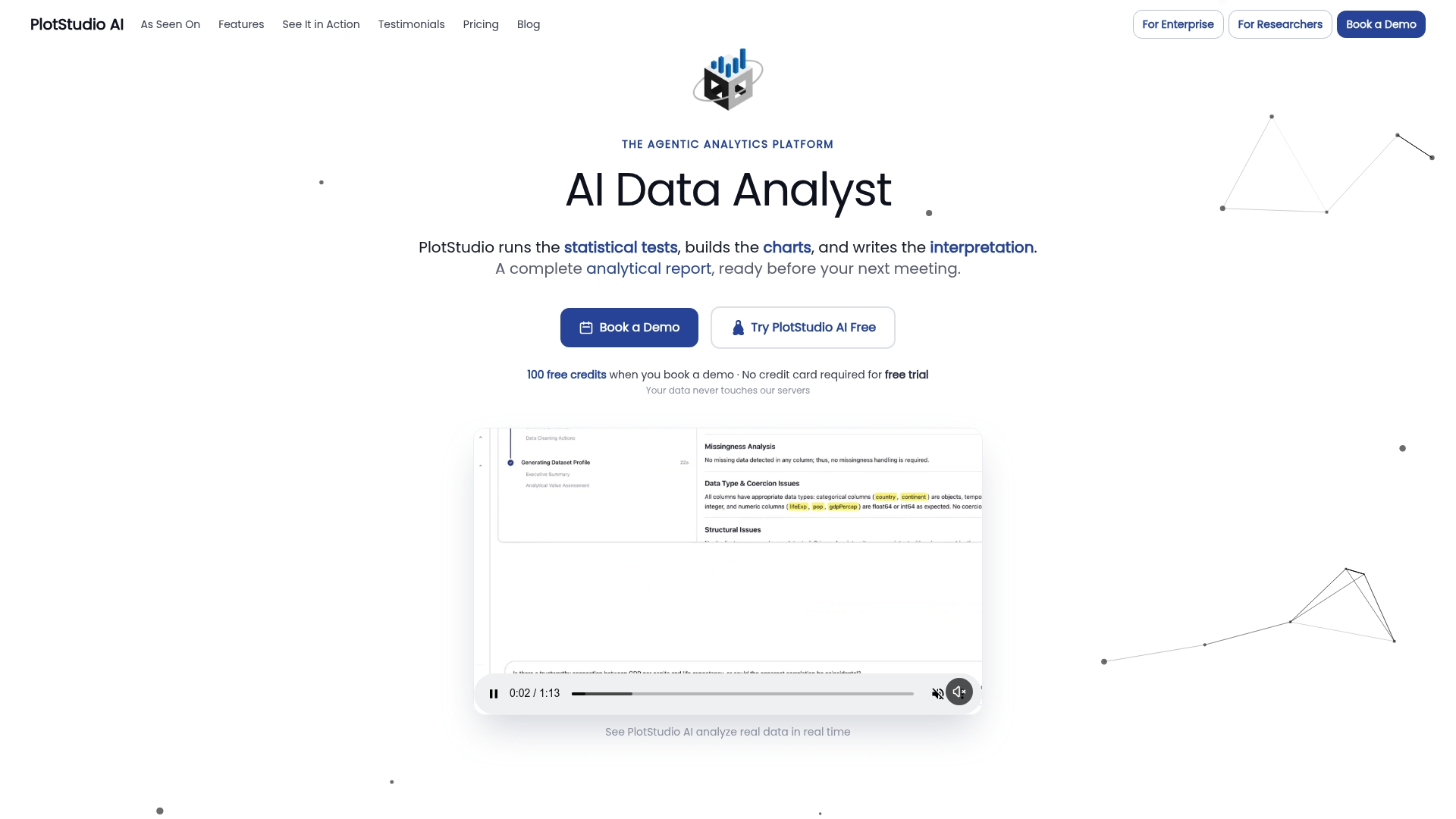
Every step covered here, stationarity tests, seasonality detection, rolling-origin validation, requires a workflow that documents itself as it runs, not one you reconstruct from memory when a reviewer asks for methods details. Plotstudio builds that audit trail into the analysis itself: you approve a plan before any code runs, and the resulting notebook, PDF report, and searchable analysis page show exactly which stationarity test, which seasonal period, and which validation window produced your result.
For labs working with sensitive longitudinal data, patient monitoring series, institutional records, anything that can’t leave the device under IRB or GDPR rules, local execution means the forecasting workflow never has to compromise on privacy to get reproducibility. Academic teams piloting a forecasting project can start through the research partnership program for credits and priority access, or review the enterprise platform details if you’re scaling forecasting across an institution or lab group.
Where to Go Deeper on Time Series Forecasting
For canonical theory, Rob Hyndman and George Athanasopoulos’s Forecasting: Principles and Practice remains the standard reference for decomposition, exponential smoothing, and ARIMA. NIST’s engineering statistics handbook covers the statistical foundations of stationarity and seasonality detection in more formal detail. For runnable code, TensorFlow’s time series tutorial and the sktime and PyTorch Forecasting documentation both offer adaptable starting pipelines.
- Explore time series analysis methods for a broader survey of modeling approaches
- Review trend analysis techniques for detrending and trend detection specifics
- Check Microsoft’s DetectSeasonality API documentation for a production example of configurable seasonality detection
Sources
- 6.4. Introduction to Time Series Analysis (NIST)
- Forecasting: Principles and Practice (oTexts)
- Time series forecasting | TensorFlow Core
- Time Series Analysis: Definition, Types, Techniques, and When It’s Used | Tableau