Time Series Forecasting Methods for Data Analysts

For most applied forecasting problems, start with three methods in sequence: seasonal-naive or ETS (Holt-Winters family) for strongly seasonal data with short histories; auto.arima (via R’s forecast package or Python’s statsmodels) when stationarity is uncertain and you need interpretable coefficients; and XGBoost with lag features when nonlinearity, many covariates, or longer histories make statistical models underfit. If you’re working at scale across many series, feature-based meta-learners like FFORMS/FFORMA can select among those methods automatically, producing near-state-of-the-art accuracy without fitting every candidate model. Deep learning (LSTM, Transformer) earns its place only when you have large, complex datasets with multiple seasonal patterns and enough compute to tune properly. Whatever method you choose, benchmark it with time-series cross-validation (rolling-origin evaluation) and keep a reproducible pipeline from day one.
- Seasonal-naive / ETS: Fast to fit, interpretable, and surprisingly hard to beat on short monthly or quarterly series.
- auto.arima: Handles differencing and order selection automatically; ACF/PACF diagnostics remain readable.
- XGBoost with lag features: Strong on nonlinear relationships and external regressors; requires careful leakage prevention.
- FFORMS/FFORMA: Meta-learning frameworks that map series features to method choices; operationally efficient at scale.
- LSTM / Transformer: Reserve for high-frequency, long-horizon problems with abundant training data.
Pro Tip: Before committing to any method, run a seasonal-naive baseline. If your candidate model can’t beat it on rolling-origin CV, the added complexity isn’t justified.
Key Takeaways
Statistical baselines (ETS, auto.arima) should be your starting point for most time series forecasting problems, with escalation to ML or meta-learning frameworks justified only by measurable cross-validated gains.
| Point | Details |
|---|---|
| Start with statistical baselines | Fit seasonal-naive and ETS first; they outperform complex models on short or moderately seasonal series. |
| Use rolling-origin CV | Rolling-window cross-validation produces more stable model comparisons than any single train/test split. |
| Escalate to ML with evidence | Add XGBoost or deep learning only when CV scores on multiple folds show measurable improvement over ETS/ARIMA. |
| Meta-learning scales selection | FFORMS/FFORMA and AutoForecast automate model choice across large series portfolios efficiently. |
| Plotstudio for reproducibility | Plotstudio enforces pre-registered analysis plans, local execution, and full audit trails for research-grade forecasting. |
Table of Contents
- What makes time series different from standard regression
- Classical statistical forecasting methods: ETS, ARIMA, and naive baselines
- Machine learning and deep-learning approaches: when they actually help
- Data prep and feature engineering that materially change forecast performance
- How to evaluate and pick forecasting models
- A decision rulebook for matching data to forecasting methods
- Building research-grade, reproducible forecasting pipelines
- Plotstudio supports reproducible forecasting for research teams
- Sources
What makes time series different from standard regression
Time series data carries structure that ordinary cross-sectional regression ignores: observations are ordered, and the distance between them in time matters. Understanding that structure before choosing a forecasting technique is what separates a defensible model from a lucky one.
Components you need to identify first
Every time series can be decomposed into a trend-cycle (the long-run direction), a seasonal component (repeating patterns tied to calendar periods), and a remainder (the residual noise after both are removed). Decomposition is a diagnostic step as much as a modeling step: it tells you whether seasonality is growing with the level of the series (multiplicative) or staying roughly constant (additive). When seasonal amplitude scales with level, use multiplicative decomposition or log-transform the series before fitting an additive model. STL (Seasonal-Trend decomposition using LOESS) is worth knowing as a flexible alternative when seasonal patterns shift over time, since classical decomposition assumes a fixed seasonal shape.
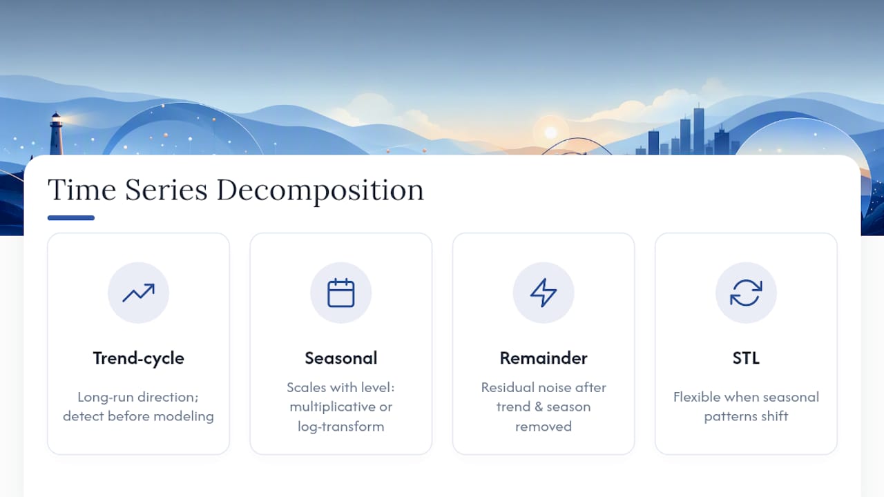
Trend-cycle detection is equally important for understanding long-run patterns before you commit to a model class.
Stationarity and why it matters
A stationary series has a constant mean and variance over time. Most classical statistical models assume stationarity, so you need to check for it before fitting ARIMA or related methods. The Augmented Dickey-Fuller (ADF) test checks for a unit root (non-stationarity); KPSS tests the null of stationarity instead, so running both gives a clearer picture. In practice, visual inspection of the series plot, ACF, and PACF often tells you as much as the formal tests.
Quick diagnostic checklist before modeling:
- Plot the raw series: look for trend, level shifts, and changing variance.
- Inspect the ACF for slow decay (trend) and spikes at seasonal lags.
- Use PACF to identify AR order candidates.
- Run a seasonal subseries plot to check whether seasonal patterns are stable.
- Apply a periodogram to detect dominant frequencies in high-frequency data.
- Test stationarity with ADF and KPSS; difference or log-transform as needed.
Pro Tip: When seasonality amplitude scales with level, prefer multiplicative treatment or log-transform before modeling. Fitting an additive ETS to a multiplicative series systematically underestimates peak values.
Classical statistical forecasting methods: ETS, ARIMA, and naive baselines
Classical methods remain the most interpretable starting point for most applied forecasting problems, and they are often the most accurate on short or moderately seasonal series.
ETS and the Holt-Winters family
ETS stands for Error, Trend, Seasonality, and the family covers 30 possible state-space model combinations. Holt-Winters is the most familiar member: it applies exponential smoothing to level, trend, and seasonal components simultaneously. The additive version suits series with constant seasonal swings; the multiplicative version handles series where those swings grow with the level. In R, ets() from the forecast package fits the full ETS family and selects the best specification by AIC automatically. Prediction intervals come directly from the state-space formulation, which is a practical advantage over many ML approaches.
ARIMA and SARIMA
ARIMA models capture autocorrelation structure through autoregressive (AR) and moving-average (MA) terms, with differencing (the “I”) to handle non-stationarity. SARIMA adds seasonal AR and MA terms and a seasonal differencing step. Identifying the right orders (p, d, q)(P, D, Q)s is the hard part: the ACF suggests MA order, the PACF suggests AR order, and the number of differences needed is guided by stationarity tests. auto.arima() in R’s forecast package automates this search using AIC/BIC over a grid of candidate models. In Python, statsmodels.tsa.statespace.SARIMAX provides equivalent functionality with support for exogenous regressors.
Naive baselines you should never skip
- Naive: The forecast equals the last observed value. Surprisingly competitive on random-walk series.
- Seasonal-naive: The forecast equals the value from the same season one period ago. A strong baseline for weekly or monthly data.
- Drift: Extends the naive forecast with a linear trend estimated from the full history.
These baselines are not just placeholders. If your model can’t beat seasonal-naive on rolling-origin CV, you haven’t justified its complexity.
Pro Tip: Use auto.arima() with stepwise=FALSE and approximation=FALSE for a thorough grid search on shorter series. The default stepwise mode is faster but can miss the global optimum.
| Method | Best for | Seasonality handling | Exogenous regressors | Interpretability | Computation cost | Horizon suitability |
|---|---|---|---|---|---|---|
| Seasonal-naive | Short series, strong seasonality | Direct seasonal copy | No | Very high | Negligible | Short |
| ETS / Holt-Winters | Monthly/quarterly, stable seasonality | Additive or multiplicative | No | High | Low | Short–medium |
| ARIMA / SARIMA | Stationary or differenced series | Seasonal terms (SARIMA) | Yes (ARIMAX) | High | Low–medium | Short–medium |
| State-space (general) | Structural modeling, missing data | Via structural components | Yes | Medium | Medium | Short–medium |
Machine learning and deep-learning approaches: when they actually help
ML methods for time series are not a universal upgrade over statistical baselines. They earn their place under specific conditions: nonlinear relationships, many external covariates, long histories, or multiple interacting seasonal patterns.
Supervised learning framing and leakage risk
The standard ML approach converts a time series into a supervised learning problem by constructing lag features (y at t-1, t-2, …, t-k) and rolling statistics as inputs, with the future value as the target. The critical risk is data leakage: if any feature is computed using information from after the forecast origin, your CV scores will be optimistic and your production model will fail. Use a strict rolling-origin split where the feature window never overlaps with the target period.
XGBoost and gradient boosting
XGBoost handles nonlinearity and categorical covariates (day-of-week, holiday flags, product category) without explicit feature transformation. It scales well to large datasets and supports missing values natively. The trade-off is that it requires deliberate feature engineering: lag selection, rolling aggregates, and calendar features all need to be constructed explicitly. Backtesting with multiple rolling-origin folds is non-negotiable before trusting XGBoost’s CV scores, because the model can overfit to a single fold’s noise pattern.

Deep learning: LSTM, GRU, and Transformers
Recurrent architectures (LSTM, GRU) and Transformer-based models capture long-range temporal dependencies that lag-feature tabular models miss. TensorFlow/Keras and PyTorch both provide well-documented implementations. The honest caveat: these models need substantial training data (typically thousands of observations per series, or a large panel of related series), significant compute, and careful hyperparameter tuning. On short or moderately seasonal series, they routinely underperform a well-tuned ETS or ARIMA. Reserve them for high-frequency data (hourly energy demand, intraday financial series) or global models trained across many related series.
Hybrid models and meta-learning
Hybrid approaches combine a statistical model’s trend/seasonality decomposition with an ML model’s residual fitting. The statistical component handles the interpretable structure; the ML component captures nonlinear residuals. FFORMS and FFORMA take a different angle: they extract features from the series (using libraries like tsfeatures or catch22) and use those features to select or weight among candidate models, producing forecasts that are nearly as accurate as state-of-the-art methods while being faster to compute. For large-scale deployments across many series, this is often the most operationally practical path.
Pro Tip: When using XGBoost for time series, always include at least one lag at the seasonal period (e.g., lag-12 for monthly data) alongside short lags. Omitting the seasonal lag is the single most common feature-engineering mistake.
- Construct lag features strictly within the training window to prevent leakage.
- Use
scikit-learnpipelines to chain feature transformers and the model; this makes retraining deterministic. - For deep models, use TensorFlow/Keras with a reproducible random seed and log all hyperparameters.
- Evaluate on multiple rolling-origin folds, not a single holdout, before comparing ML against statistical baselines.
- Consider AI forecasting tool alternatives when evaluating operational deployment options beyond custom model code.
Data prep and feature engineering that materially change forecast performance
A well-specified model on poorly prepared data will underperform a simpler model on clean data. These steps consistently matter.
Handling missing and irregular data
Before any model fitting, audit the series for gaps. Impute short gaps with linear interpolation or forward-fill; flag longer gaps with a binary missingness indicator so the model can learn that those periods are unreliable. For irregular intervals, resample to a consistent frequency using aggregation (sum or mean, depending on the measure) before modeling. Outliers deserve explicit treatment: winsorize at the 1st/99th percentile or model them as additive outliers in a state-space framework rather than silently dropping them.
Feature engineering checklist
- Lag values: y(t-1), y(t-2), …, y(t-k); include the seasonal lag (e.g., t-12 for monthly).
- Differences: first difference, seasonal difference, and their interaction.
- Rolling statistics: rolling mean, rolling standard deviation over windows of 3, 7, 14, or 28 periods.
- Calendar features: hour-of-day, day-of-week, week-of-year, month, public holiday flags.
- Fourier terms: sine/cosine pairs at dominant seasonal frequencies; useful for complex or multiple seasonalities.
- Exogenous regressors: promotions, weather variables, economic indicators — anything with a causal relationship to the target.
For intermittent demand (many zeros, irregular spikes), standard ETS and ARIMA perform poorly. Croston’s method and its variants (Syntetos-Boylan approximation, TSB) are designed specifically for this pattern. Inventory forecasting applications illustrate how intermittent-demand methods reduce overstock in supply chain contexts.
Pro Tip: Standardize your feature pipeline and persist all transformers (scalers, encoders, lag constructors) as serialized objects. At inference time, load the same transformer objects used during training. Rebuilding transformers from scratch at inference is a common source of subtle data drift.
| Feature type | Implementation | When it helps most |
|---|---|---|
| Seasonal lag (t-s) | Direct lag at period s | Any series with clear seasonality |
| Fourier terms | forecast::fourier() in R; manual sin/cos in Python |
Multiple or complex seasonalities |
| Rolling mean (window w) | pd.Series.rolling(w).mean() |
Smoothing noisy series, trend proxies |
| Holiday flags | pandas holiday calendars; timeDate in R |
Retail, energy, transport data |
| Missingness indicator | Binary flag at gap positions | Series with irregular gaps |
How to evaluate and pick forecasting models
Choosing a model without a rigorous evaluation workflow is the fastest way to deploy something that looks good in development and fails in production.
Metrics and their trade-offs
- MAE (Mean Absolute Error): Robust to outliers; interpretable in the original units. Use it as your primary metric when outliers are common.
- RMSE (Root Mean Squared Error): Penalizes large errors more heavily; useful when large misses are disproportionately costly.
- MAPE (Mean Absolute Percentage Error): Intuitive as a percentage, but undefined when actuals are zero and biased toward under-forecasting.
- sMAPE (Symmetric MAPE): Addresses MAPE’s asymmetry; still problematic near zero.
- MASE (Mean Absolute Scaled Error): Scales by the in-sample naive forecast error; comparable across series of different scales and the preferred metric in M-competition evaluations.
Avoid relying solely on AIC for model selection; combine information criteria with cross-validated error and structural checks to guard against instability from structural breaks.
Time-series cross-validation (rolling-origin)
Rolling-origin evaluation produces more stable model assessments than a single train/test split. The procedure: fix a minimum training length, generate forecasts from each origin, advance the origin by one period (or one batch), and average the error across all origins. This mirrors how the model will actually be used in production.
Backtesting checklist:
- Set a minimum training window (at least two full seasonal cycles for seasonal models).
- Define the forecast horizon you care about (h=1, h=12, etc.) and score at each horizon separately.
- Advance the origin by one period per fold; use at least 10–20 folds for stable estimates.
- Average the chosen metric across folds before comparing model classes.
- Check stability: a model that is slightly worse on average but consistent across folds often outperforms a volatile winner in production.
- Fit the selected model class to the full available history for final deployment.
Automated model selection: FFORMS, FFORMA, and AutoForecast
Feature-based frameworks extract characteristics from the series (length, strength of trend, seasonality, spikiness, entropy) and use those features to select or weight among candidate models. A decision-tree-based feature-driven framework applied to the M3 dataset demonstrated that assessing 22 series characteristics across seven forecasting methods can reliably identify an adequate model without exhaustive fitting. AutoForecast takes this further with temporal meta-learning, reporting a large median inference-time reduction compared to naive selection approaches in experimental testbeds. For teams managing hundreds or thousands of series, that speed difference is the practical argument for meta-learning over manual selection.
For forecasting accuracy trade-offs across metrics and model classes, the key principle is to score every candidate on the same rolling-origin folds before declaring a winner.
A decision rulebook for matching data to forecasting methods
The right method depends on five variables: series length, data frequency, seasonality type, availability of exogenous data, and forecast horizon. Work through them in order.
Prioritized escalation path
Start simple and escalate only when CV scores justify it:
- Step 1: Fit seasonal-naive and ETS as baselines. Score on rolling-origin CV.
- Step 2: Add ARIMA/SARIMA if stationarity tests suggest autocorrelation structure beyond ETS.
- Step 3: Introduce XGBoost with lag and calendar features if nonlinearity or many covariates are present.
- Step 4: Apply FFORMS/FFORMA for automated selection across many series, or ensemble the top two CV performers.
- Step 5: Escalate to LSTM or Transformer only if high-frequency data and large training sets are available and CV gains are measurable.
Special cases worth calling out
Intermittent demand (many zeros, irregular spikes): use Croston’s method or the Syntetos-Boylan approximation rather than ETS or ARIMA, which assume a continuous process.
Multiple seasonalities (e.g., daily and weekly patterns in hourly data): use TBATS, Prophet, or Fourier-term extensions of ARIMA/ETS. Prophet handles multiple seasonalities natively and supports holiday regressors, making it practical for business time series with irregular calendar effects.
Multivariate forecasting (multiple related series): VAR (Vector Autoregression) models capture cross-series dynamics; panel data methods extend this to large panels with shared structure. Global ML models (a single XGBoost trained across all series) often outperform per-series models when series share common patterns.
Building research-grade, reproducible forecasting pipelines
A forecast that can’t be reproduced is a forecast that can’t be defended. For academic work, grant applications, or any analysis subject to peer review, reproducibility is not optional.
Step-by-step reproducible pipeline
- Pin your environment: use
renv® orconda/piplock files (Python) to record exact package versions. - Document data provenance: record the source, extraction date, and any preprocessing applied to the raw data before it enters the pipeline.
- Pre-register your analysis plan: specify the model classes to evaluate, the CV procedure, the primary metric, and the decision rule for model selection before running any code.
- Code all transforms: never apply manual edits to data files; every imputation, outlier treatment, and feature construction must be scripted.
- Version your models: save fitted model objects with a timestamp and the training data hash; never overwrite a production model without archiving the previous version.
- Archive outputs: store forecasts, CV scores, and prediction intervals alongside the code that produced them.
Audit signals that matter in production
- Seed control: set and log random seeds for any stochastic step (train/test splits, neural network initialization, bootstrap intervals).
- Saved transformers: serialize all scalers, encoders, and lag constructors; load them at inference rather than recomputing.
- Deterministic scoring: confirm that running the evaluation script twice on the same data produces identical metric values.
- Prediction-interval calibration: check empirical coverage (what fraction of actuals fall within the stated 95% interval) at each retraining cycle.
- Drift monitoring: track sMAPE or MAE on a rolling window of recent actuals; a sudden increase signals a structural break or data quality issue.
Pro Tip: *Schedule a model audit at every major retraining cycle: re-run rolling-origin evaluation on the most recent data window and compare CV scores to the baseline established at deployment.
FFORMS/FFORMA-style meta-learning fits naturally into reproducible pipelines: precompute the feature-to-model mapping offline, serialize it, and run a single-model fit online. This preserves competitive accuracy while keeping inference fast and the pipeline auditable.
Practical forecasting also requires operational steps beyond model fit: scheduled retraining, monitoring for drift, and documented retraining triggers are what sustain performance after deployment.
What experienced practitioners actually learn from forecasting projects
The most consistent lesson from real forecasting work is that simpler models win more often than practitioners expect, especially early in a project. An ETS or ARIMA fitted on clean data with a well-chosen seasonal period will outperform a poorly specified LSTM on the same data in the majority of cases. Complexity must be justified by measurable CV gains, not by the appeal of the method.
The operational failures that cause the most damage are rarely about model architecture. Data leakage is the most common: a feature computed on the full dataset before the train/test split, or a rolling statistic whose window bleeds into the target period. It produces CV scores that look excellent and production performance that collapses. The second most common failure is a mismatched retraining cadence: a model trained on annual data being asked to forecast weekly patterns without retraining, or a model retrained too infrequently to track a structural shift in the series.
Prediction intervals are the most consistently ignored output in applied forecasting. Analysts report the point forecast and treat the interval as a footnote.
The M-competitions (M1 through M5) have repeatedly shown that simple methods and ensembles of simple methods are hard to beat on diverse real-world series. That finding should recalibrate how much time you spend on architecture search versus data quality and feature engineering.
Plotstudio supports reproducible forecasting for research teams
Researchers who need defensible, auditable forecasting workflows face a specific problem: most cloud-based tools require uploading sensitive data, and most general-purpose analytics platforms don’t enforce pre-registration or reproducibility standards.
Plotstudio runs analysis locally on your machine, so IRB-governed, GDPR special-category, or otherwise sensitive time series data never leaves your device. Every forecasting analysis is gated behind an analysis plan you review and approve before any code runs, functioning as a pre-registration and an audit trail. R and Python both run natively, which means auto.arima, ets(), statsmodels, XGBoost, and TensorFlow/Keras workflows all execute within the same reproducible environment. Outputs include annotated notebooks, PDF reports, and permanent searchable analysis pages that a supervisor or reviewer can trace end-to-end.
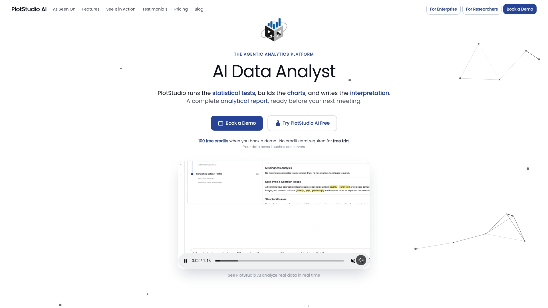
For academic teams and research partnerships, Plotstudio offers free credits and priority access through its research partner program, and discounted academic pricing for university researchers. If you’re evaluating it as a purpose-built alternative to general analytics tools, the advanced data analysis alternative page details the full capability set.
Sources
Core textbooks and online resources:
- Decomposition — Forecasting: Principles and Practice (OTexts)
- Forecast model selection – Rob J Hyndman
Software documentation and tutorials: