Why can the same dataset yield a mostly explained gap in one paper and a mostly unexplained one in the next? The Blinder Oaxaca decomposition splits a mean outcome gap between two groups into an endowment part, the share associated with different average characteristics, and a coefficient part, the share associated with different estimated returns. The raw gap is fixed. The split is not.
Two decisions drive that instability: which coefficients you use to price characteristics, and which variables enter the model at all. A published decomposition that leaves both unstated isn't reproducible, only suggestive.
What the Blinder Oaxaca Decomposition Measures
Start with the quantity you can observe. Let A be one group, B the other, and let Δ be the difference in mean outcomes, mean of A minus mean of B. The decomposition asks a counterfactual question: how much of Δ would remain if the two groups had identical average characteristics, and how much exists because the same characteristic is priced differently in each group. A Census Bureau Center for Economic Studies working paper writes the gap as the sum of an endowment effect and a coefficient effect evaluated at a chosen reference coefficient vector.
Take a wage gap. Men in your sample earn more per hour than women. Education and experience differ on average, and pricing that difference at the reference returns gives the endowment effect. What's left over is the coefficient effect: men and women may earn different returns per year of education, and their intercepts may differ, which surfaces as a baseline gap that no measured covariate explains.
Why a Reference Vector Is Unavoidable
You can't price a difference in characteristics without a price list. The endowment term is the mean covariate gap multiplied by β*, and nothing in the data hands you β*. You choose it: the men's coefficients, the women's coefficients, a pooled regression, or a reweighted structure. That makes the decomposition an accounting identity rather than an estimator with a unique answer.
The threefold version isolates the interaction term on its own line, because unequal characteristics and unequal returns arrive together. Read the components in order and you get a clean narrative: different inputs, different prices, and the overlap between them.
What Each Component Is Allowed to Mean
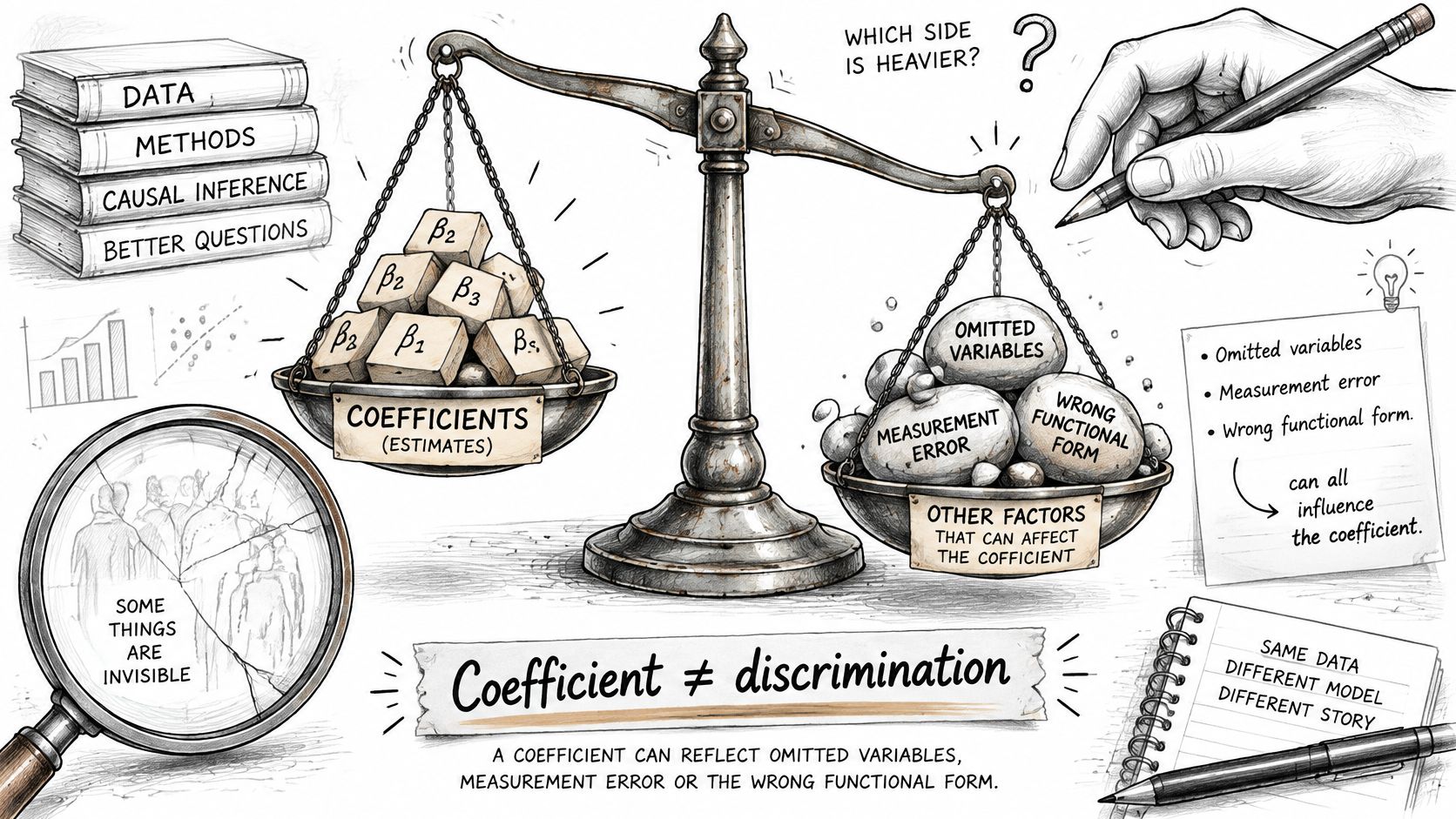
The coefficient term is a statistical residual. It can reflect discrimination, and it can equally reflect omitted variables, measurement error, model misspecification, or genuine structural differences in how the two groups sort into jobs. The working paper is explicit that the decomposition is descriptive, and that "associated with" is the honest verb until identification assumptions justify stronger language.
Keep this table next to the code while writing up, because it forces the wording to match the component.
| Component | Formula term | What it measures | How to phrase it |
|---|---|---|---|
| Total mean gap | Mean of A minus mean of B | Observed difference in average outcome | Report as the starting gap |
| Endowment (explained) | (X̄A minus X̄B) times beta star | Gap associated with different average characteristics | Associated with differences in education and experience |
| Coefficient (unexplained) | X̄A times (betaA minus beta star) plus X̄B times (beta star minus betaB) | Gap associated with different returns, including intercept differences | Residual association, not automatically discrimination |
| Interaction (threefold only) | (X̄A minus X̄B) times (betaA minus betaB) | Joint effect of unequal characteristics and unequal returns | Reported as its own component |
The Assumptions the Split Rests On
Four conditions hold up the arithmetic. Linearity: each group's conditional mean outcome is linear in the covariates, so the fitted returns describe that group. A deliberate reference: β* is stated and justified, never inherited from a software default. Overlap: both groups contain observations across the relevant covariate range, so the counterfactual is interpolation rather than extrapolation. No unmeasured group-specific confounder: nothing omitted from the model shifts outcomes differently for the two groups.
Break any of them and the coefficient component still means something, but only as an association measured under that specification. It stops being a number you can attach to a cause.
Phrasing rule: write "associated with" in every sentence about the coefficient component until your design earns something stronger. Reviewers forgive hedging. They don't forgive overclaiming.
Common Variants and Their Assumptions
Pick the variant before you write a line of code, because each one adds an assumption you'll have to defend in the methods section.
| Variant | What changes | Assumptions added | Trade-off |
|---|---|---|---|
| Twofold | One reference coefficient vector splits explained and unexplained parts | Linear conditional means and common support | Allocation shifts with the reference |
| Threefold | Adds an interaction term for characteristics and returns together | Same as twofold | Interaction must be reported as its own component |
| Pooled-coefficient | Reference is one model with a group indicator | Shared returns across groups | Check specification against group-specific fits |
| Reweighted (Oaxaca-Ransom) | Weights align covariate distributions across groups | Common support after weighting | Needs weight and overlap diagnostics |
| Nonlinear (Fairlie) | Binary or count outcomes with a counterfactual on the outcome scale | Correct link and functional form | Component sizes depend on the link function |
| Machine-learning estimators | Flexible models relax linearity | Weaker functional-form assumptions | Reference choice still needs sensitivity checks |
The twofold split is the default because it's the easiest to explain and the hardest to misread. The threefold version earns its extra line when you expect the interaction to be large, and a Springer-published methodological note on the threefold decomposition makes the useful point that the interaction isn't an additional control-variable effect. It's the joint presence of unequal endowments and unequal returns, and folding it into either side of the split misreports both.
Binary outcomes behave differently enough to deserve their own paragraph. The counterfactual has to be computed on the probability scale, so component sizes depend on the link function and the numbers read as percentage-point contributions. A 2025 study of Argentine manufacturing firms, published by Springer Nature, reported a predicted probability of technological innovation of 0.943 for firms cooperating in R&D and 0.6381 for non-cooperating firms, an Oaxaca-Blinder gap of 30.52 percentage points. That's the kind of quantity a probability-scale decomposition produces, and it isn't interchangeable with a coefficient from a linear probability model.
Whatever you choose, name its assumptions and run the twofold result alongside it. Readers need to see what the variant changed.
Selecting Covariates Before Estimation
The model you fit decides the answer as much as the estimator does. Choose covariates by theory and timing before you touch either group regression, and write the reason for each inclusion next to the variable name.
The rule that trips people up is the mediator. Occupation is the obvious case in wage work: women are concentrated in lower-paid occupations, so occupation sits on the path from group to outcome. Control for it and part of the gap you wanted to measure gets absorbed, and the explained share falls. The same logic applies to hours worked, firm size, or sector in other literatures.
- Check timing first: education completed before labour-market entry belongs in the model; a promotion earned after the gap opened usually doesn't.
- Model curvature deliberately: include experience and its square where returns are nonlinear, then check residual plots by group instead of trusting the R-squared.
- Treat blocks consistently: industry or region dummies need one reference category, coded identically in both groups.
- Screen for collinearity: education, experience, and tenure overlap, and near-collinear terms make returns unstable enough that small data changes move the component sizes.
- Avoid padding: a long list of weakly relevant controls shifts both components and inflates the variance of the group coefficients.
Covariate choice is one of the two decisions that move the split. The other is the reference structure, and recent methodological work shows that changing the reference group can reverse the sign of either component and produce substantively different conclusions about which group is disadvantaged (arXiv preprint on reference-group dependence). That's the practical reason to document covariates before estimation and revisit them alongside the reference sweep.
If you're shaky on how adding a variable changes a coefficient at all, the guide to multiple regression covers omitted variable bias and the mechanics of added controls before you extend them to a two-group split.
Choosing the Reference Coefficients That Shape the Result
The total gap doesn't move when you change the reference. Only the split does, and sometimes it moves far enough to change your conclusion.
The structure is ΔY = (X̄A − X̄B)′β* + [X̄A′(βA − β*) + X̄B′(β* − βB)], where the first bracketed term is the explained component and the second is the unexplained component under that reference. Because β* also decides where the threefold interaction lands, the oaxaca_blinder crate documentation describes this as the index-number problem and argues it should be reported explicitly rather than treated as a mechanical detail.
| Reference | Coefficients used | When it fits | Trade-off |
|---|---|---|---|
| Group A structure | betaA | Group A is the baseline for the policy question | Allocation changes if the groups are swapped |
| Group B structure | betaB | Group B is the baseline for the policy question | Mirror-image allocation, so check both directions |
| Pooled structure | beta star from pooled regression with a group indicator | Neither group is treated as the norm | Imposes shared returns, so check the specification |
| Reweighted structure | Group A or B coefficients applied to reweighted covariates | Covariate distributions overlap well after weighting | Needs common support and weighting diagnostics |
Run the decomposition twice, once under each group's coefficients, and read the pair together. When the higher-paid group's returns are used to price everyone's characteristics, the endowment term tends to swell and the coefficient term shrinks. Take the other group's returns as the norm and the accounting mirrors. Neither version is wrong, and the data can't choose between them on its own.
One decomposition is a single draw from a set of defensible specifications. Report the range.
The sweep I run before submission: re-estimate under each reference structure and with the groups swapped; vary the covariate sets and the functional form, with and without the squared experience term; trim non-overlapping observations and rerun on the common-support sample; and for nonlinear outcomes, rerun with the alternative estimator. Tabulate the explained and unexplained shares with confidence intervals across every run.
If the explained share moves widely across reasonable specifications, the headline depends on the specification, and the paper should say so. If the sign of a component flips, report the decomposition as descriptive and drop any directional claim about which group benefits.
Running the Decomposition Step by Step
The sequence below is what I'd hand a student, with the check that has to pass before the next step.
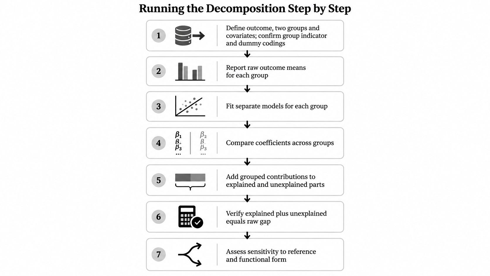
- Fix the objects. Define the outcome, the two groups, and the covariates, and confirm the group indicator and dummy codings are consistent across the dataset. Check that group counts equal the sample sizes you'll report.
- Fit two regressions. A separate linear model per group, outcome on covariates, with an intercept. Check that coefficient signs match theory before going further.
- Compute the raw gap. Group mean outcomes, group mean covariates, and the difference. Check the gap against a plain t-test of group means.
- Build the counterfactual. Group A's mean characteristics evaluated at group B's coefficients, or the reverse, under the reference you've chosen. Check that the counterfactual predicted mean falls inside the observed range, not beyond it.
- Split and reconcile. Explained plus unexplained must equal the raw gap exactly. A residual mismatch almost always means an intercept or dummy-coding error.
- Attach uncertainty. Delta method or bootstrap, with both group regressions re-estimated in every resample. Clustered or heteroskedastic data need the same treatment here as anywhere else, which is why the notes on robust standard errors apply directly.
- Go detailed. Break the explained component down by covariate and look for large positive and negative contributions that cancel. An aggregate explained share can hide a big offsetting pair.
The Stata Journal article by Ben Jann describes the conventional setup: separate linear regressions per group, then a comparison of the observed mean difference with counterfactual predicted means. It also states the caveat plainly. The residual contains omitted variables, measurement error, misspecification, unobserved characteristics, and functional-form error, so the method decomposes a statistical gap rather than establishing a causal discrimination effect.
Three slips account for most of the broken sum checks: a dropped intercept in the counterfactual, a sign convention that flips between the two groups, and components reported without the sum check at all.
When the Decomposition Can and Cannot Be Trusted
A large coefficient component is the most over-read result in applied social science. It means the gap survives equalizing measured characteristics. It does not mean differential treatment caused the gap.
The two deeper threats get far less airtime than the discrimination misreading, and both can invalidate the whole exercise.
Unobserved Confounding
Ordinary least squares decompositions can omit productivity-relevant factors and leave endogeneity unaddressed, which biases both the regression coefficients and the resulting attribution of the gap. The oaxaca package vignette warns directly that the unexplained portion may reflect unobserved variables rather than discrimination. Recent work proposes weighted or doubly-protected estimators with trimming, or orthogonal machine-learning methods, to handle common-support and misspecification problems.
Common Support
If one group's covariate profiles barely occur in the other group, the counterfactual is extrapolation rather than comparison. Say nearly all women in a sample have under five years of tenure and nearly all men have over fifteen. At fifteen years, the counterfactual for women comes from a region of the covariate space where women barely appear. The model will still return a number. It just won't be a comparison.
If the counterfactual requires covariate values the data never contain, you don't have a decomposition. You have a projection.
Diagnostics to Run Before Interpreting
- Overlap plots: covariate distributions by group, inspected variable by variable.
- Propensity-score or covariate-support checks: flag regions where one group is thin or absent.
- Trimming sensitivity: rerun on the common-support sample and see how much the shares move.
- Alternative specifications: different covariate sets, functional forms, and references.
- Confidence intervals: the literature notes that applications often omit standard errors and intervals entirely, which limits how much the reported shares can bear.
The Go or No-Go Rule
If overlap is poor, trim or reweight, and say so in the text. If the specification is unstable, present the result as descriptive only and remove causal verbs from the abstract.
When the question is causal rather than accounting, the decomposition isn't the right tool. A causal inference analysis design answers a different question under different assumptions, and mixing the two vocabularies in one paper is where most overclaiming starts.
Worked Example in R and Python
What happens when you run the same wage gap through two different tools? Take a wage extract with a binary gender indicator, log hourly wage, years of education, potential experience, and tenure. The workflow differs by language, but the arithmetic must agree.
| Task | R (oaxaca package) | Python (statsmodels) |
|---|---|---|
| Fit group models and decomposition | oaxaca with a formula that places the group variable after the vertical bar | Two OLS fits, then group means and counterfactual predictions by hand |
| Reference coefficients | Set by the package options for the reference structure | Written explicitly in the code for each reference |
| Bootstrap inference | Replicate count passed as an argument | Loop that resamples rows and recomputes the components |
| Output to check | Components with standard errors and confidence intervals | A table of components that must sum to the raw gap |
In R With the oaxaca Package
The formula puts the group variable to the right of the vertical bar, as in lnwage ~ educ + exper + tenure | female. Pass the bootstrap replicate count as an argument rather than accepting whatever the default is, and read four things from the output: the aggregate components, their standard errors, the confidence intervals, and the detailed contributions by covariate.
The detail table is where the paper's story usually lives. Education often contributes little to a contemporary gender gap, tenure contributes moderately, and the intercept carries a large share of the residual. That intercept pattern is worth flagging early, because reviewers ask about it.
In Python With statsmodels
Core scientific Python has no single canonical routine for this, so you fit two OLS models, pull the group means, and compute the counterfactual prediction yourself. It's more verbose. It's also the version where every assumption is visible in the code, which matters if a coauthor wants to audit the reference choice.
Write the three components into a dataframe with a column recording which reference produced them. When you later run the reference sweep, you append rows rather than rewriting the script. That small habit is what turns a single number into evidence about how fragile the number is.
Reading the Two Outputs Against Each Other
The sum check is the same in both. Explained plus unexplained must reproduce the raw gap to numerical precision. If R and Python disagree, the cause is nearly always coding: a dropped intercept, a different reference, or a dummy set with mismatched base categories.
Then write the interpretation in three sentences. State which component is larger, what the larger one is associated with in substantive terms, and what the reference choice implies about the range. The honest version looks like this: the coefficient component carries most of the gap under men's returns, the split changes when women's returns are used as the reference, and the explained share therefore isn't identified by the data alone. Watch for the case where the two shares change direction across references, because that is the finding, not a nuisance to hide in a footnote.
If you'd rather spend your time on that paragraph than on rebuilding the plumbing, the walkthrough on R programming for statistical analysis covers the surrounding workflow, from data checks to exporting a table.
Report Your Decomposition So Reviewers Can Check It
A decomposition earns its place in a paper only when a reviewer can rebuild it from the write-up alone. The checklist below is what research reproducibility looks like for a two-group decomposition.
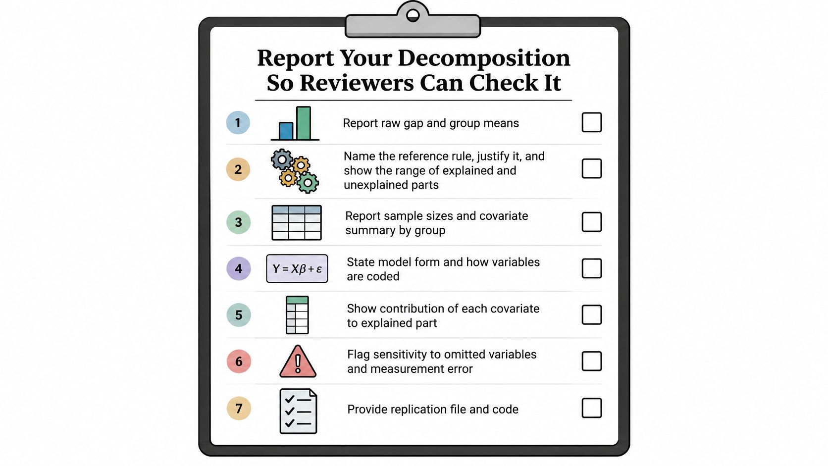
- Report the raw gap and both group means before any decomposition figure appears. A reader who cannot see the starting point cannot verify that explained plus unexplained sums back to it.
- Name the reference rule and justify it, then show the explained and unexplained shares under each alternative you tested. If the shares swap size or change direction across references, say so, because that range is the honest answer to how much of the gap the covariates account for.
- Give every component a confidence interval, with the inference method and the number of bootstrap replicates stated. The documented R implementation defaults to 100 replicates when no value is supplied (oaxaca vignette), so report your count rather than leaving readers to assume one.
- Spell out covariate coding and intercept treatment, including detailed contributions and any positive and negative terms that offset. The ddecompose package documentation lists the same core requirements: raw gap, exact reference rule, variable coding, component estimates with intervals, and sensitivity to alternative weighting schemes.
- Use "associated with" language for the coefficient component unless the identification strategy supports more.
- Keep the cleaning log with the analysis. PlotStudio AI's cleaner documents every transformation, including row counts dropped, imputations, and recodings, so the audit trail a reviewer asks for already exists.
Run the reference and sensitivity checks once more before submitting the table. The item most likely to draw a question is the counterfactual: which group's returns were used to price the characteristics. A reviewer who sees the sweep reported already has the answer.
If you would rather spend the afternoon on interpretation than on stitching together R output, Python output, and a cleaning log, PlotStudio AI runs the analysis and saves it as a reproducible Analysis Page with the underlying code attached.