R Programming for Statistical Analysis: A Practical Guide

R programming for statistical analysis doesn't require an add-on package for every test: the built-in R stats package already supports statistical calculations and random-number generation. The harder work is choosing a model that matches your study design, checking what could invalidate it, and preserving enough of the environment for another researcher to reproduce your conclusions.

How to Set Up R for a Reproducible Analysis

Set up a project-specific environment, not just an R installation. The R Project describes R as free software for statistical computing and graphics on UNIX, Windows, and macOS, with support for linear and nonlinear modeling, classical tests, time series, classification, and clustering. That breadth lets you keep data preparation, estimation, diagnostics, and reporting in one executable workflow.

Use the following setup before exploring your dataset:

1. Match the R version. Install the version your collaborators use when continuing an established analysis. Record it rather than assuming everyone's current installation is equivalent.
2. Connect your editor. Install RStudio or another IDE and confirm that it uses the intended R binary. An editor upgrade and an R upgrade are separate changes.
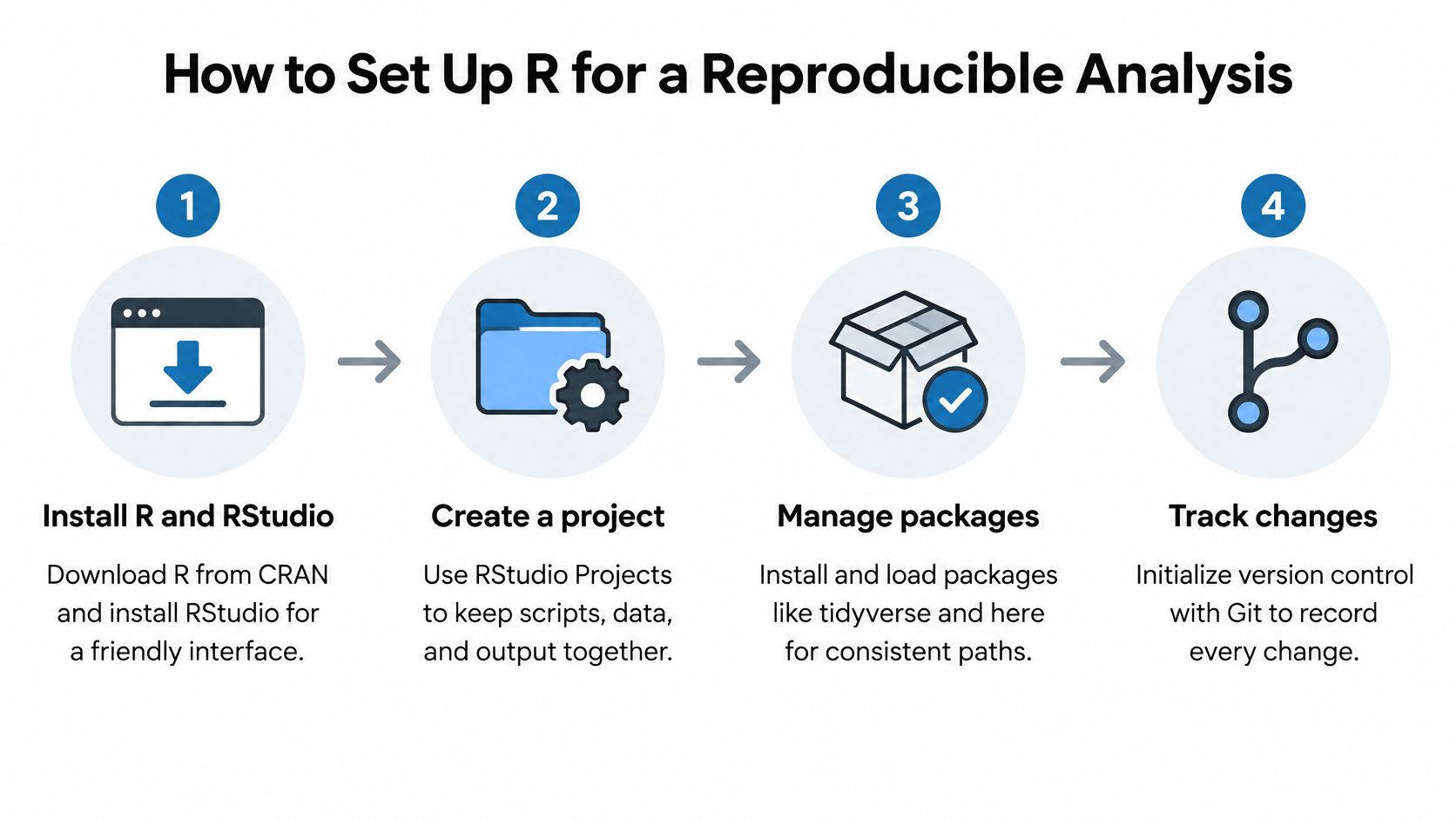
3. Create a project. Use an RStudio Project and project-relative paths such as data/raw/trial.csv. Avoid setwd() calls containing your personal home directory.
4. Isolate dependencies. Run renv::init() to establish a project library. After installing and testing the required packages, run renv::snapshot() to record their versions in renv.lock.
5. Capture the session. Save sessionInfo() with writeLines(capture.output(sessionInfo()), "session-info.txt").
6. Control randomness. Put a documented set.seed() call before simulations, bootstrapping, or resampling. Record parallel random-number settings when applicable.
7. Separate inputs and outputs. Keep original files read-only in data/raw, derived datasets in data/processed, and generated reports in an output folder.

This process flow summarizes the project structure and version-control habits.

Check for environment drift

Run renv::status() before handing the project to a collaborator. Resolve differences between the installed library and the lockfile deliberately, rather than automatically snapshotting an unexplained change.

Use Git to track scripts, the lockfile, and documentation, but don't commit confidential participant data. A lockfile also doesn't capture every operating-system dependency or external tool needed to render a report.

Practical rule: A project that runs only in your current interactive session isn't ready for handoff.

Treat the research reproducibility checklist as a way to identify missing inputs, undocumented dependencies, and hidden manual steps.

Packages That Cover Each Stage of an R Analysis

Packages by analysis stage

Analysis stage	Package	Use it for
Data wrangling	dplyr, tidyr (tidyverse)	Filter, group, join, and reshape tables
Large tables	data.table	Fast grouped operations on millions of rows
Plotting	ggplot2	Layered, publication-ready figures
Tidy model output	broom	Model results as data frames for reports
Mixed models	lme4	Random intercepts and slopes for repeated or clustered data
Survival analysis	survival	Kaplan-Meier curves and Cox models
Post-hoc comparisons	emmeans	Estimated marginal means and pairwise contrasts
Regression diagnostics	car	Variance inflation factors and Type II or III tests
Locked dependencies	renv	Reinstall the package versions used in the original analysis

The official introduction to R distinguishes the base environment, standard and recommended packages, and contributed extensions. Packages add specialized methods without requiring a different language, but installing a package doesn't establish that its method fits your question.

Let base R and specialist packages split the work

Base R is a sensible starting point for summaries, classical tests, linear models, and quick diagnostic plots. The tidyverse makes chained transformations easier to inspect when you're joining files, grouping observations, and reshaping repeated measurements.

For example, tidyr::pivot_longer() can turn visit-specific columns into a longitudinal table. That transformation changes the table's shape, not the independence of its observations. The participant identifier must survive the reshape so the model can represent within-person dependence.

Use data.table when table size or repeated grouped operations justify it. Don't rewrite a readable analysis solely because another package has a reputation for speed. For performance-critical work, the bench documentation supports benchmarking elapsed time, CPU time, memory allocation, and garbage collection on representative expressions.

Inspect interfaces before trusting results

• Name functions explicitly. Write dplyr::filter() when function masking could cause confusion.
• Read model-specific help. broom::tidy() formats supported model output, but it doesn't make different coefficient scales interchangeable.
• Check contrasts. emmeans comparisons depend on the fitted model, reference grid, weighting, and multiplicity adjustment.
• Keep reporting separate. Use Quarto for the document and packages such as gt or modelsummary for tables generated from analysis objects.

More packages mean more dependencies to restore and more defaults to understand. Match the outcome and design to the method first, install the smallest useful package set, and run the help examples before adapting them to your study.

How to Import, Clean and Profile Data in R

Define the estimand, the quantity you want to estimate, and identify what a row represents before cleaning. A participant, a clinic, a plot, and a participant visit aren't interchangeable observational units. Keep a cleaning log that connects every transformation to a reason.

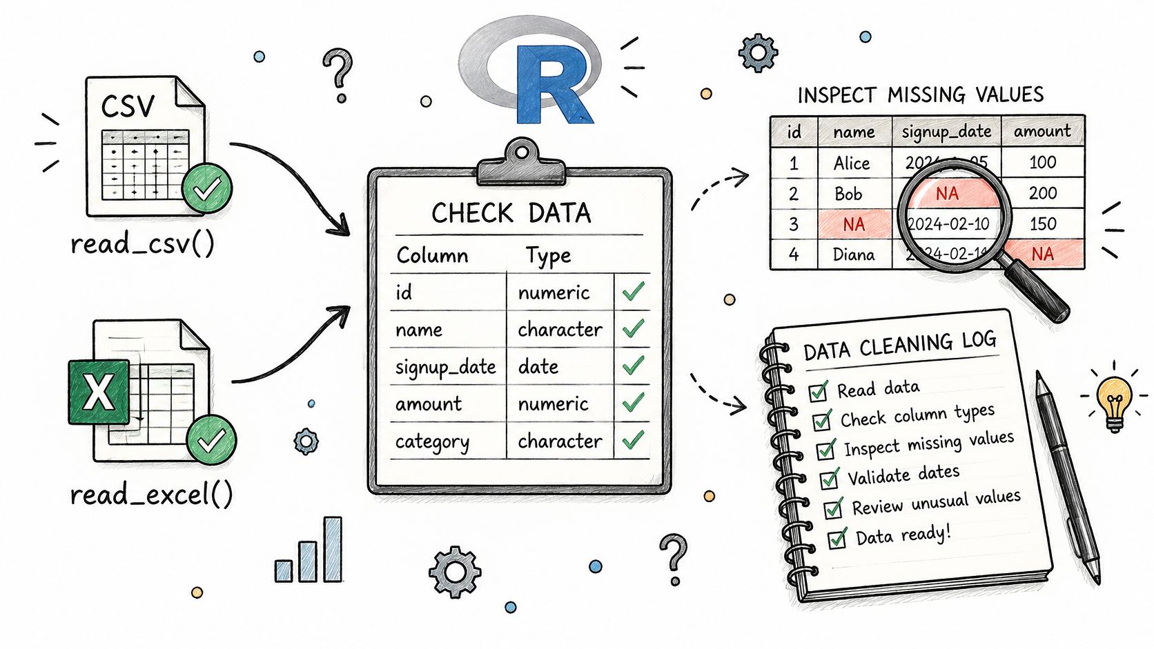
The illustration summarizes the import-to-validation sequence.

Make each check leave evidence

1. Declare types. For a CSV, use readr::read_csv() with col_types = readr::cols(id = readr::col_character(), treatment = readr::col_character(), outcome = readr::col_double()). Character identifiers preserve leading zeros. For Excel, set col_types in readxl::read_excel().
2. Inspect structure. Run str(df) or dplyr::glimpse(df), followed by summary(df). Check parsing problems rather than suppressing warnings.
3. Count missingness. colSums(is.na(df)) reveals incomplete columns. Compare these counts with visit schedules and the codebook.
4. Check duplication. duplicated(df) finds identical rows. Also inspect the intended key, such as participant and visit, because conflicting duplicate records won't necessarily be identical.
5. Validate values. Use range(df$outcome, na.rm = TRUE) and table(df$treatment, useNA = "ifany") to catch implausible measurements and inconsistent labels.
6. Record transformations. Recode with dplyr::mutate() and save row counts before and after exclusions or joins.

The R manuals provide the underlying documentation for data handling, statistical functions, and script-based workflows. For import troubleshooting, the guide to reading a CSV file in R addresses the practical entry point.

Nested instrument exports or API responses may not fit a rectangular CSV cleanly. Fetchin's explanation of when to use JSON over CSV helps distinguish file-format decisions from subsequent statistical cleaning.

Investigate missingness before replacing values

In a longitudinal trial, missing outcomes after withdrawal may have a different explanation from an accidentally skipped measurement. Missing completely at random, missing at random, and missing not at random describe different assumptions; observed data alone generally can't settle which explanation is correct.

Don't convert missing outcomes to zero. Likewise, sum(x, na.rm = TRUE) omits missing values, but doesn't establish that the resulting total is scientifically meaningful. Avoid blindly converting factors with as.numeric(), which can return internal category codes.

Plot the outcome with hist() or ggplot2::geom_histogram(), then inspect treatment relationships with geom_boxplot() or geom_point(). Record skew, outliers, and unequal spread without automatically deleting unusual observations.

For a complementary walkthrough of R data-analysis mechanics, use the video below.

Choosing and Checking a Model in R

Design and outcome to R function

Data and design	Test or model	R function	Package
Continuous outcome, two independent groups	Welch t-test	t.test()	stats
Continuous outcome, three or more groups	One-way ANOVA	aov()	stats
Continuous outcome, repeated measures	Linear mixed model	lmer()	lme4
Binary outcome	Logistic regression	glm(family = binomial)	stats
Time to event	Cox proportional hazards	coxph()	survival
Count outcome	Poisson or negative binomial	glm(family = poisson), glm.nb()	stats, MASS

Treat this table as a starting point, not an automatic selector. One-way ANOVA assumes an appropriate independent-error structure and common residual variance; a mixed model needs a defensible random-effects structure. Counts may require an exposure offset, while survival analysis requires attention to censoring and proportional hazards.

Tyson Barrett's guidance on common R pitfalls emphasizes understanding assumptions and exploring data before modeling. Reducing coding friction doesn't establish statistical validity.

Specify the scientific comparison

Say a genotype trial measures yield across blocks. If blocks represent a sampled source of variation and the design supports that treatment, lme4::lmer(yield ~ genotype + (1 | block), data = trial) represents block-level dependence.

That formula isn't a universal agricultural model. Repeated seasons, spatial structure, or genotype-by-environment questions may require different terms. A random intercept also won't automatically capture every longitudinal correlation pattern.

Choose covariates using the design and scientific question, not a search for whichever adjustment produces significance. An adjusted association isn't automatically causal, and prediction requires validation on observations that weren't used to tune the model.

Make diagnostics change decisions

• Curved residual patterns. For a linear model, inspect residuals against fitted values with plot(model). Consider a scientifically justified transformation or spline rather than ignoring nonlinearity.
• Unequal residual spread. Consider heteroskedasticity-consistent inference through sandwich, paired with an appropriate coefficient-testing function. The guide to robust standard errors explains the distinction between changing uncertainty estimates and changing the fitted mean.
• Influential observations. Examine hat values and cooks.distance(model). Check measurement provenance before considering exclusion.
• Collinearity. Inspect car::vif(model), remembering that multi-parameter terms may produce generalized VIFs. Large values warrant investigation, not automatic deletion.
• Model-specific failures. Check overdispersion for count models and survival::cox.zph() for Cox models. A normal Q-Q plot isn't a universal diagnostic for every outcome family.

For sensitivity analysis, compare the prespecified result with a justified alternative, such as a model excluding a verified questionable measurement. Report whether the substantive conclusion changes.

A sensitivity analysis tests dependence on a defensible choice. It isn't permission to keep the version with the smallest p-value.

When screening many hypotheses, define the testing family and consider p.adjust(p_values, method = "BH"). Label exploratory findings, and report effect sizes with intervals from confint() or the appropriate model-specific method, not p-values alone.

Exporting Reproducible Reports and Figures

Code sharing isn't the same as a successful rerun. A study of R projects on the Open Science Framework examined 296 projects, found 98.8% lacked formal dependency descriptions, and reported that only 25.87% of reconstructed projects completed execution without errors. Build a handoff that tests execution rather than merely making files available.

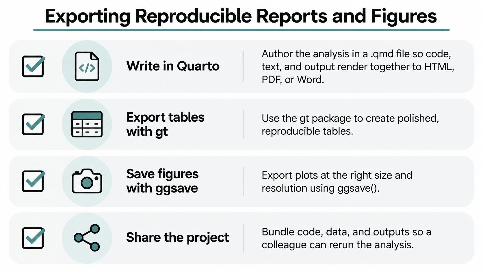
Use this checklist to connect the manuscript to its analytical artifacts.

Generate outputs from objects

1. Author in Quarto. A .qmd document keeps code, interpretation, and results together for HTML, PDF, or Word rendering. Document additional rendering dependencies, including those needed for PDF.
2. Build tables programmatically. Use gt or modelsummary instead of retyping estimates. This prevents a revised model from leaving obsolete values in the manuscript.
3. Fix figure specifications. Call ggplot2::ggsave() with explicit width, height, units, and resolution. Use manuscript-aligned filenames and check the exported file, not just the IDE preview.
4. Preserve analytical objects. Use saveRDS() for fitted models, derived datasets, and reference estimates. Saved objects support inspection but don't replace executable source code.
5. Write a README. State the run order, required inputs, expected outputs, and any authorized data-access procedure.

Apply data visualization best practices to scales, labels, and uncertainty displays. Reproducibility preserves a chart faithfully; it doesn't make a misleading chart appropriate.

Test the handoff in a clean session

Restore dependencies with renv::restore() in a clean checkout, then run the complete pipeline without loading objects from your interactive workspace. Compare regenerated estimates against saved reference values with all.equal() using a documented tolerance.

If estimates differ meaningfully, investigate input files, package versions, random-number generation, numerical libraries, and model convergence. Don't assume every discrepancy is a seed problem.

Submission check: Resolve unexplained differences before sending the manuscript, even when both runs produce statistically significant results.

For restricted data, share the access instructions and a suitable test dataset where permitted. Never imply a colleague can reproduce an analysis without access to its required inputs.

Questions Researchers Ask About R

Is R free for statistical analysis?

Yes. R's source code was released under the GNU General Public License in 1995, according to the R project history presented by Kurt Hornik. You can use the language without purchasing a proprietary statistical-software license.

Do researchers still use R, and how does it compare with Python?

Yes, but journal use, survey responses, and popularity rankings measure different things.

Where R shows up in 2025 surveys

Source	R figure	Comparison
Soil-science journal study, reported 2025	7,899 of 25,888 articles in 10 journals, published from 2014 to 2023, named R as the primary tool, 30.5%	Published-use measure, not a Python comparison
Kaggle Data Science Survey analysis, 2025	5,335 R users, 20.54% of respondents included in the calculation	Survey-use measure
Account of the 2025 Stack Overflow Developer Survey	4.9% of respondents used R	57.9% used Python
Report on the December 2025 TIOBE index	Ranked 10th at 1.96%	Popularity index, not research usage

Prefer R when the required method is well supported in CRAN or Bioconductor and your lab maintains R scripts. Prefer Python when the surrounding project centers on general programming or an established Python pipeline. Popularity isn't a method-selection criterion.

Which R function should I use for my statistical test?

Identify the outcome, observational unit, dependence structure, and target comparison first. Use a statistical test selection framework to narrow the options, then inspect assumptions and package defaults before interpreting output.

Can someone else rerun my R analysis?

Only if they can obtain the necessary inputs and reconstruct the execution environment. The Quarto file, lockfile, documented randomness, data provenance, and external dependencies must form a complete package. A report that renders successfully without rerunning cached calculations doesn't demonstrate a fresh execution.

Hand Off One Analysis This Week

Choose an analysis you already trust and test its portability. A result you believe in gives you a reference point: if the rebuilt run diverges, the environment broke something. Keep the exercise narrow, because pairing it with a new model search or a large rewrite makes discrepancies harder to diagnose.

Use a bounded acceptance test

• Prepare a clean project. Initialize its environment and connect the script to the preserved raw input.
• Run the prespecified model. Save the target coefficients, uncertainty estimates, and diagnostics as reference artifacts.
• Rebuild elsewhere. Restore dependencies on another machine or clean environment and compare regenerated results with all.equal().
• Investigate mismatches. Check data identity, dependencies, randomness, and convergence before accepting the handoff.

Matching estimates support the numerical handoff. They say nothing about whether the scientific assumptions still hold, so treat a clean rebuild as the minimum bar for reproducibility.

Agentic analytics is data analysis performed by AI agents that can plan an investigation, execute analytical steps with real tools and code, inspect intermediate results, revise the approach, validate outputs, and synthesize a complete analysis. The researcher still judges the estimand, assumptions, and sensitivity checks.

---

Once the R handoff succeeds, download and try PlotStudio AI for a complementary investigation that executes Python locally on your machine. PlotStudio AI saves Analysis Pages containing the generated code and a written description of each step; its cleaner documents every dropped row, imputation, and recoding, and results export to a PDF report or a Jupyter notebook. Use those inspectable artifacts to judge the work: an answer is an output; an analysis is an investigation.