No clustering algorithm wins every dataset. Eleven methods compared across five datasets produced no consistent leader on any of three evaluation perspectives, and DBSCAN's Adjusted Rand Index has run from 0% at default parameters to 100% once its neighborhood settings were varied.
The most popular advice on this topic is to start with k-means and let silhouette score pick the winner. The first half is defensible when the geometry fits. The second half will get a result past you that shouldn't pass, because silhouette rewards convex, evenly sized groups, which is the exact shape k-means is built to produce. Any ranking built that way flatters one family by construction.
A comparison of clustering algorithms is a model-selection problem with at least five objectives: fit quality, runtime, peak memory, how noise is handled, and stability under reseeding or resampling. The table below narrows the field in one pass. Everything after it is about defending whichever candidate survives.
A Decision Table for Clustering Algorithms
A comparison of clustering algorithms comes down to four facts about your file, not a universal ranking: the geometry of the groups, whether some points should stay unassigned, how many rows and columns you have, and whether k is known before you fit. Fix those four and the candidate list collapses to two or three methods worth running.
| Algorithm | Shape it assumes | Noise | Scale | Main controls | Use it when |
|---|---|---|---|---|---|
| K-means | Compact, similar-sized, roughly spherical | No outlier label, centroids drift toward extremes | Strong, linear in n | k, initialization, feature scaling | Groups are even and n is large |
| Mini-batch k-means | Same as k-means | Same centroid sensitivity | Best runtime and memory of the common set | k, batch size | Millions of rows and a rough partition is acceptable |
| Ward hierarchical | Compact, nested groups | Early merges are hard to undo | Weak, about three times the runtime of k-means at 5,000 records | Linkage, cut height or k | A dendrogram is the deliverable and n is modest |
| DIANA | Divisive hierarchy | A split is hard to reverse | Poor for large n | Stop rule or k | You need a top-down split, not a fast partition |
| PAM | Arbitrary shape via medoids | More robust than means | Slow, use CLARA when n is large | k, distance | Outliers or a non-Euclidean distance matter |
| DBSCAN | Arbitrary shape, similar density | Labels sparse points as noise | Good with a spatial index, weak on huge n | eps, min_samples | Irregular groups and explicit outliers |
| OPTICS | Arbitrary shape, varying density | Reachability plot exposes noise | Slower than DBSCAN | min_samples, xi | Density changes across clusters |
| HDBSCAN | Varying density, hierarchical | Excess-of-mass extraction drops noise | Moderate | min_cluster_size | You want DBSCAN-like clusters without tuning eps |
| Gaussian mixture | Elliptical, overlapping | A component can absorb outliers | Moderate, EM cost grows with components | Components, covariance type | Membership should be a probability |
| Spectral | Non-convex or manifold structure | Sensitive to affinity and noise | Up to about twice the time and 30 times the memory of mini-batch k-means | k, neighbors or bandwidth | Structure is non-convex and n is not huge |
The table generates a shortlist; it doesn't settle anything. A 2022 comparison published in ACM Computing Surveys evaluated 11 clustering algorithms (K-means, PAM, CLARA, hierarchical and agglomerative clustering, decisive clustering, DBSCAN, OPTICS, SOTA, expectation-maximization, and Fanny) on Iris, College, Wine, US Arrests, and WWW Usage, judged three ways: external validation against known labels, internal compactness and separation, and stability under changes to the data or the initialization. No single method dominated across all datasets and criteria.
Where the density rows earn their place
The review is specific about both edges of DBSCAN. It was judged appropriate for large datasets holding unevenly sized or arbitrarily shaped groups, because clusters expand from dense regions and sparse observations can be labeled outliers instead of absorbed into a group. The failure cases are just as concrete: performance degrades when cluster densities vary substantially, when two clusters are joined by a narrow neck, and when the dataset grows very large.
Scan the table in a fixed order and you'll stop shopping. Start with shape, which most PCA or pairwise plots will answer in a minute. Then ask whether a noise label is scientifically necessary, since that single requirement removes every partitioning and hierarchical method from the list. Then check scale, because a spectral or Ward fit on a million rows isn't a choice, it's an outage. Controls come last.
Model selection, not model shopping: treat the table as the set of candidates you owe an argument to, then let the machine learning model selection workflow govern how you compare them.
What Each Algorithm Family Assumes
Every family encodes a definition of a cluster, and the definition is what fails when the data disagrees with it.
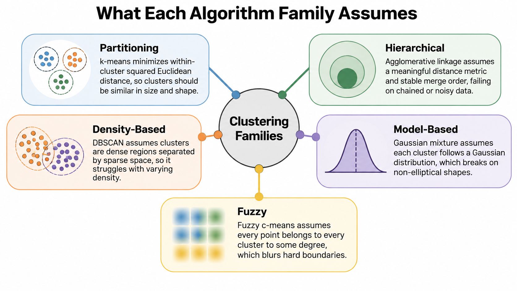
Partitioning methods minimize within-cluster squared Euclidean distance, which asserts that groups are similar in size and variance. Change k, change the initialization to k-means++, or run several random seeds, and you get a different partition and a different answer to whether the first one was stable. Medoids replace the mean with a real observation, so an extreme row can't drag the center of a cluster across the plot, and you can supply any distance you like, at a cost several times higher than means.
Hierarchical methods build a tree. Ward merges pairs to minimize the variance added at each step; DIANA splits from the top down. The tree is the scientific object, which is also the weakness: a bad merge in the first fifty steps can't be repaired by the cut you choose at the end.
Density methods grow clusters where a neighborhood of radius eps contains at least min_samples points. OPTICS orders points by reachability so a single eps stops being a requirement, and HDBSCAN extracts the branches that persist across a range of density levels, which makes it the practical default when density is uneven.
Model-based and graph-based close the set. A Gaussian mixture fitted by expectation-maximization permits elliptical covariance and soft membership, though a full covariance with too many components will overfit a few hundred rows. Spectral clustering embeds a similarity graph and partitions the embedding, which recovers rings and moons that k-means slices through the middle. Fuzzy c-means relaxes the hard assignment by giving each point a membership in every cluster, which blurs boundaries rather than resolving them.
Three scaling facts decide more fits than any algorithmic preference. Euclidean methods need standardized features, because a column measured in thousands will outvote a column measured in tenths. A prechosen distance in PAM does not inherit that scaling. And hierarchical memory grows with the square of n, so a file that fits fine on your laptop can strand a cluster job.
Before fitting anything, plot a sample in the first two principal components and answer one question: do the groups look round, nested, dense, overlapping, or wrapped around a gap?
Quality Runtime and Parameter Sensitivity
The highest quality score can be the least defensible result if it comes at the cost of runtime, memory, or stability. The scikit-learn guide's artificial benchmarks show why method choice depends on several objectives at once.
| Result | Figure | Comparison | Source setting |
|---|---|---|---|
| Mini-batch k-means | Best combined accuracy, runtime, and memory | Against spectral, DBSCAN, and regular decomposition | Artificial benchmarks in the scikit-learn clustering guide |
| Spectral clustering | Up to 2× time and 30× memory | Against mini-batch k-means, with competitive ARI | Same artificial benchmarks |
| DBSCAN at defaults | ARI as low as 0% | Many untouched parameter settings | Same artificial benchmarks |
| DBSCAN after tuning | ARI as high as 100% | Almost all tested artificial experiments once parameters varied | Same artificial benchmarks |
| K-means runtime | 3.5 seconds | 5,000 records | 2025 college-management study, ACM |
| Hierarchical runtime | 11.2 seconds | Same 5,000 records | 2025 college-management study, ACM |
In the artificial benchmarks summarized in the scikit-learn clustering documentation, mini-batch k-means had the strongest combined result across accuracy, runtime, and memory. Spectral clustering remained competitive on Adjusted Rand Index, but used up to 2 times the time and 30 times the memory. That trade-off may be justified when its partition better matches the structure under study; otherwise, the extra cost buys little.
Read the DBSCAN row twice
With many default parameter settings, DBSCAN's ARI fell to 0%. After varying neighborhood parameters, it reached 100% in almost all tested artificial experiments. The gap shows how strongly the result depends on configuration. A report that gives only the default run cannot establish that density-based clustering failed.
Runtime depends on the dataset and implementation, but a same-size comparison makes the cost concrete: the cited study reports 11.2 seconds for hierarchical clustering and 3.5 seconds for k-means on 5,000 records. The roughly threefold difference may be acceptable when a dendrogram is part of the analysis. For a fast partition, it is a meaningful penalty.
Report the grid, not the verdict: a claim that DBSCAN failed is incomplete without eps, min_samples, the distance, and the scaling.
Compare methods across distinct costs: quality, wall-clock time, peak memory, noise handling, and stability across seeds. Record measurements on the dataset at hand. A high score on one run does not establish a reliable partition if small changes in initialization produce different assignments.
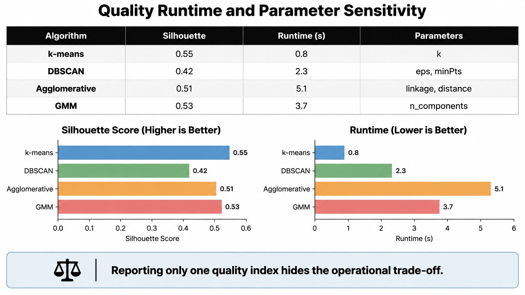
The highest ARI is not automatically the most defensible choice. A slower method that changes substantially across seeds may be less useful than a faster, repeatable partition with a slightly lower score.
Metrics Hyperparameters and a Worked Check
Validation is where a plausible partition becomes a defensible one, and it takes three numbers, not one.
Silhouette runs from -1 to 1, and higher means a point sits closer to its own cluster than to the nearest other one. Davies-Bouldin is a ratio of within-cluster spread to between-cluster separation, so lower is better. Calinski-Harabasz is a variance ratio, so higher is better. Adjusted Rand Index sits near 0 for chance agreement and 1 for perfect agreement with known labels; use Adjusted Mutual Information when two labelings differ in granularity.
A 2025 study compared clustering algorithms against expert-generated groups and reported silhouette scores of 0.387 for K-means, 0.377 for Ward, 0.342 for DIANA, 0.405 for PAM, 0.133 for DPC, and 0.042 for DBSCAN (Springer, 2025). Read that line as a lesson about index bias rather than a ranking. DBSCAN's 0.042 partly reflects an index that penalizes noise labels and irregular density, which are the two properties DBSCAN was selected to produce.
Preprocessing moves the same index just as far. In a 2025 student-learning-behavior experiment published in ACM conference proceedings, an improved K-means procedure raised silhouette from 0.421 to 0.484 and cut the Davies-Bouldin index from 1.83 to 1.46. The gain came from the pipeline around the algorithm, not from a new family.
The check, in five steps
- Scale only what needs scaling. Standardize features whose units differ and leave already-comparable measures alone.
- Choose k with three signals. The elbow, the silhouette curve, and a domain maximum you can defend in a sentence.
- Fit two families that can disagree. K-means and HDBSCAN on the same representation is a genuine test, because they define a cluster differently.
- Report a profile. Silhouette plus one separation index plus stability across at least ten seeds, with noise plotted as its own symbol.
- Add ARI only if labels exist, and never tune parameters on the labels you later score against.
Keeping the code short helps: StandardScaler, KMeans or AgglomerativeClustering, HDBSCAN, and silhouette_score, with the seed and the parameter grid printed above the figure. Internal scores choose among fits of a sensible family. They don't prove the clusters are real groups.
Research Scenarios That Change the Choice
Scenarios pick the family. Metrics only confirm it.
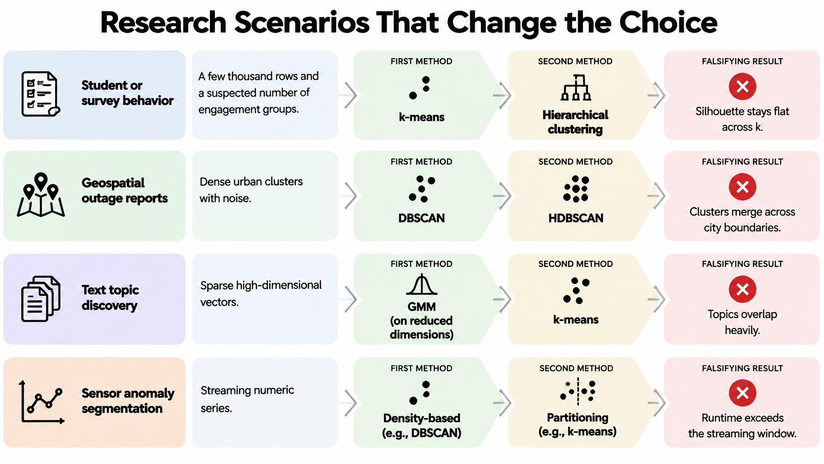
A few thousand survey rows with a suspected number of engagement groups. Start with k-means on scaled features and hold Ward as the runner-up, because a nested typology often describes student behavior better than a flat label does. The choice is falsified if silhouette stays flat across k, which means the continuum has no natural cut. Document scaling and initialization here: the improvement in a learning-behavior experiment came from exactly those choices, not from a new algorithm. A quick exploratory data analysis pass before fitting will tell you whether the continuum is even worth cutting.
Administrative records around 5,000 rows. In the 2025 college-management study published through ACM, k-means clustered 5,000 records in 3.5 seconds while hierarchical clustering took 11.2 seconds. K-means is the operational default at that size; hierarchical is justified only when leadership needs the merge tree and not just the labels.
Segments with outliers and unequal group sizes. Customer spend and lab values both produce long right tails that pull a centroid. Prefer PAM or HDBSCAN, and plot medoid profiles or a condensed tree rather than a scatter colored by label. The choice is falsified if the outlier decision changes the count of groups you report.
High-dimensional counts, such as single-cell data. Community detection on a k-nearest-neighbor graph is the first choice, with a Gaussian mixture on principal components as the runner-up. Run a modality check before generalizing, because a method stable on transcriptomic data can move on proteomic data. Use UMAP for display and never as proof.
The plot that settles arguments: a dendrogram for a hierarchical fit, a condensed tree for HDBSCAN, component ellipses for a mixture. Each shows the assumption you made instead of hiding it.
Limits of a Single Cluster Score
A high score survives less scrutiny than it appears to.
Standard comparisons rank methods by quality while underreporting runtime, peak memory, scalability, noise sensitivity, and repeatability. Single-cell benchmarking across transcriptomic and proteomic datasets found community-detection methods used relatively little memory and time and were less sensitive to increasing cell counts, deep-learning methods carried substantial time overhead, and classical machine-learning methods showed the largest fluctuations in memory and runtime as datasets grew (single-cell benchmarking, 2025). "Which clustering algorithm is best" is therefore malformed unless it names resource constraints, dataset scale, modality, and tolerable instability.
Three scientific limits matter more than any benchmark. Clusters are not causal types: a survey typology may only be slicing a continuum into labels. Labels used to compute ARI can't simultaneously serve as the discovery claim. Missing values and batch effects can manufacture the densest region in a plot, which is why anomaly detection methods belong in the same conversation as clustering, since a "cluster" of unusable rows is often an artifact of how you cleaned.
When pooling is the hidden assumption
Multi-site research adds a constraint that centralized benchmarks ignore. A 2025 federated multi-view k-means study describes clustering across local clients while preserving database privacy on large datasets, and related work identifies gradient inversion as a privacy risk in clustered federated learning, proposing gradient-free similarity measurement plus peer validation (IEEE Transactions on Mobile Computing). Unequal site sizes, non-IID samples, and fairness requirements change which algorithm is legitimate, not just which is fast.
Differential privacy and secure multiparty computation reduce utility and can shift fairness outcomes, so protection isn't free. A cluster that appears only after pooling may be a finding your study design cannot support.
Publish the runner-up when it's more stable or cheaper. Reviewers trust a comparison that names its second choice.
The fits can be automated. The decision about whether the groups answer the question cannot.
Choose a Shortlist and Keep the Record
A defensible clustering choice records what each candidate optimizes and what it costs. Keep five decisions in the analysis record:
- Define the output: flat segments, a hierarchy, noise labels, or membership probabilities.
- Screen shape assumptions against the feature space and the distance measure. A PCA or pairwise plot can reveal a mismatch, but cannot establish that a method is appropriate on its own.
- Fit at least two plausible candidates and record their settings: cluster count or minimum cluster size, epsilon or xi, covariance, linkage, scaling, and random seed, as applicable.
- Compare the trade-offs. Prefer the simpler fit only when its quality, runtime, memory use, noise assignments, and stability remain acceptable for the research question. Record any stability checks or precommitted external checks used to choose between candidates.
- Archive code, settings, and the rejected alternative using a research reproducibility checklist. Naming the runner-up and explaining why it lost makes the decision auditable.
Four practical choices still need explicit treatment. Fit clustering on scaled features or a documented distance, then use UMAP for display rather than treating its embedding as the analysis space. Record how missing values were handled before scoring, since dropping rows or imputing values can change the groups. A Gaussian mixture may suit overlapping, elliptical groups when membership probabilities matter; k-means answers a different question. Report a rejected method by name, with its settings and the reason it was less suitable.
PlotStudio AI is an agentic analytics tool for researchers. Its agents plan an investigation, write and run Python locally, inspect results, and save an Analysis Page; the documented transformations let you review how the data was changed. Explore PlotStudio AI for a dedicated analysis workspace.