Choosing a prettier chart isn't the main challenge in financial data visualization. The task is to encode prices, returns, exposures, and risk so readers can compare magnitude, time, and context without reading every cell. A useful figure answers a defined question on a shared scale, with its measurement definition, uncertainty, and data lineage attached.
What a Finance Chart Is Supposed to Show
Say you're comparing an equity fund with a bond benchmark. The equity fund finishes higher, but its investors endured a deeper decline along the way. A chart of ending values answers who finished ahead. It doesn't answer whether the additional return justified the risk.
That distinction separates a useful finance chart from a persuasive but incomplete one. Begin with the decision, then choose the measurement.
The goals come before the marks
A finance chart usually serves these goals, in this order:
- Show change: Make a return path, drawdown, or liquidity contraction visible.
- Compare entities: Put funds, issuers, or scenarios on a common baseline.
- Show structure: Explain how capital or risk is distributed across a portfolio or balance-sheet hierarchy.
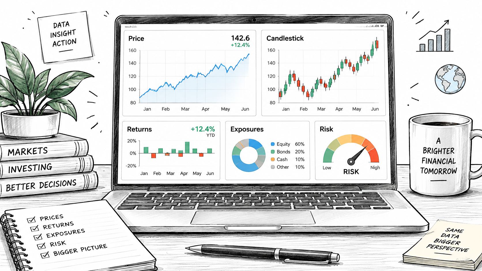
The workspace may contain many displays, but each figure needs a clear analytical purpose.
A historical analogy helps. Charles Joseph Minard's campaign map, published in 1869, represented approximately 422,000 soldiers at the outset and about 10,000 returning, a reduction of roughly 97.6%. Its band width was proportional to troop numbers, while the composition connected army size with route, direction, and retreat temperature.
This wasn't a market chart. Its lesson for finance is proportionality plus context: readers could see cumulative loss without losing the conditions surrounding it.
A vivid figure can still be the wrong comparison. Accuracy starts with what you choose to measure, not how cleanly you draw it.
That choice belongs within the broader process of financial data analysis. Chart selection, encoding, uncertainty, and the ability to rebuild the result are connected checks on the same argument.
Chart Types for Each Finance Question
| Finance question | Preferred chart | Primary encoding | Watch-out |
|---|---|---|---|
| Price or total-return path | Line chart | Position over time | Label log versus linear; shade drawdowns separately |
| Open-high-low-close session | Candlestick | Body and wick | Use only if all four prices are the question |
| Cross-section of returns or ratios | Ranked dot plot or bar | Shared baseline position | Sort against a named benchmark |
| Distribution of returns | Histogram or violin | Bin or density | State the bin rule; tails can dominate the mean |
| Correlation across assets | Diverging heatmap | Color centered at zero | Pattern only; print coefficients in a table |
| Portfolio or capital hierarchy | Treemap | Area equals weight | Add a table for close weights |
| VaR, forecast, or stress loss | Interval or fan chart | Position plus band | Label horizon, confidence, and scenario |
Choose the row from the question, not from the software's default gallery. A line chart of a total-return index answers how reinvested wealth changed. A line chart of an unadjusted share price answers a different question, even if the shapes look similar.
Candlesticks are useful when within-session movement matters. For researchers unfamiliar with their components, The Coin Course's technical analysis explained with examples provides context for reading trading displays. Recognizing a visual pattern doesn't establish that it predicts future returns.
Choose the comparison before the display
Suppose you're comparing forecast errors across issuers. Use a ranked dot plot, with the error definition and benchmark named. A bubble chart adds an unnecessary area judgment when the decision concerns which error is larger.
For a portfolio, however, a treemap can reveal broad concentration and nested sector membership. It isn't a substitute for a table when readers must distinguish similar weights. The task has changed from estimating an individual value to recognizing structure.
Distribution charts need similar care:
- Histogram: Document how bin widths and boundaries were selected. Check whether a different reasonable binning changes the apparent shape.
- Violin: State the density bandwidth rule. Smoothing can conceal isolated observations or suggest structure unsupported by the sample.
- Tail detail: Keep extreme observations visible, and inspect them before labeling them errors. A crash observation may be central to the risk question.
Time structure changes the question
A correlation heatmap compresses many pairwise relationships into a convenient overview. Calculate its cells from aligned observations, identify the return frequency, and disclose how missing pairs were handled. Otherwise, adjacent cells may summarize different samples.
For longitudinal work, time-series analysis methods help distinguish trend, dependence, and forecasting questions. A smooth line alone doesn't tell you whether observations are independent or whether an apparent relationship survives a different evaluation window.
Refuse pie slices, bubbles, or three-dimensional marks when exact comparison is the job. More elaborate marks don't compensate for a missing denominator, an unsuitable benchmark, or an undefined return measure.
Scales Labels and Annotations That Stay Quantitative
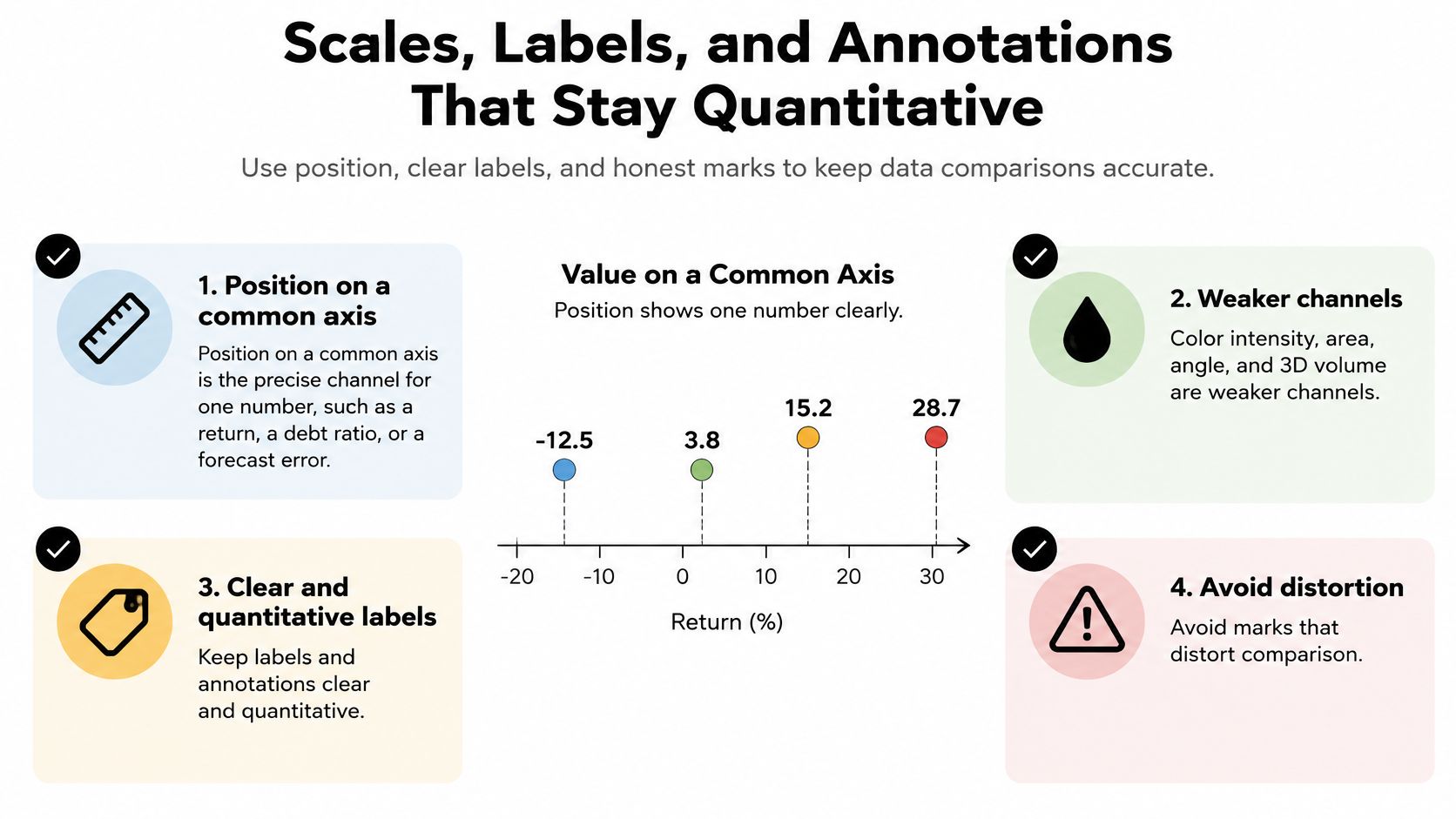
Position on a common axis should carry the main number. If researchers must compare a return, debt ratio, or forecast error precisely, don't make them infer it from circle size or color darkness.
The review The Science of Visual Data Communication finds that position supports more precise identification of individual values, while intensity can be useful for aggregate judgments. That's a reason to distinguish an exact-reading chart from a pattern-scanning display.
Use this checklist to separate measurement from decoration.
Make the primary encoding explicit
A reliable arrangement uses position for the estimate, color as a redundant sign or category cue, and a band for a defined range. Readers should still understand the main comparison in grayscale.
- Amount bars: Start at zero because readers interpret bar length as magnitude.
- Line charts: A tighter range can expose relevant movement, but make the limits conspicuous.
- Log scales: Use them when proportional change is the question and the values permit the transformation. Equal vertical distances then represent equal ratios, not equal currency differences.
- Benchmarks: Draw and label the reference readers should compare against, rather than leaving them to infer it.
A log scale doesn't turn a price series into a return series. Nor does indexing unlike assets to a common starting value make their volatility or liquidity comparable.
Put definitions where readers look
Place currency, units, sample window, and adjustment status near the title. Specify whether a return is cumulative or annualized, nominal or inflation-adjusted, and before or after fees when those distinctions apply.
Direct labels reduce repeated trips to a legend. An adjacent table preserves exact values in a publication, while hover values can supplement an interactive version. Neither should be needed to discover what the metric means.
Practical rule: Ask a colleague to identify the measurement mark, the reference mark, and the uncertainty mark. If they can't distinguish them, simplify the figure.
For an additional visual explanation, use the video alongside the checklist rather than instead of the written definitions.
Avoid a second vertical axis unless a stated identity links the scales, such as a transparent unit conversion. Independently rescaling unrelated series can make slopes appear aligned without a meaningful quantitative relationship.
Keep event annotations sparse. Add the date and a short explanatory clause only when the event changes interpretation, such as a restatement affecting comparability. Temporal proximity alone isn't evidence that the event caused the movement.
Uncertainty Bands Horizons and What They Do Not Promise
A shaded region is ambiguous until you name what it represents. Financial data visualization needs to distinguish uncertainty about an estimate from variation in outcomes.
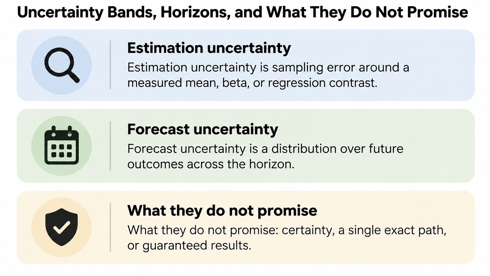
- Estimation uncertainty: Sampling uncertainty around a measured mean, beta, or regression contrast.
- Forecast uncertainty: A distribution over future outcomes at a stated horizon.
- Outcome variability: Dispersion in realized observations or paths, including historical drawdowns.
A narrow interval around an estimated average doesn't mean individual outcomes cluster tightly around it. A historical range also isn't automatically a forecast interval.
Explain what the band contains
Every band needs a horizon, calculation method, confidence level or scenario definition, and a plain-language limitation. State that the midpoint isn't a target and the band isn't a promise.
For an estimated mean return, explain that the interval concerns the average under the stated model and sampling assumptions. For a forecast, explain which future quantity is covered and which drivers were held fixed. A guide to understanding confidence intervals can help researchers avoid treating parameter uncertainty as individual outcome variability.
Time dependence matters. Resampling individual observations as though returns were independent can misrepresent uncertainty when dependence is material. Use a method appropriate to the data structure, document its assumptions, and inspect sensitivity to the evaluation window.
Test the decision, not just the drawing
The IEEE study of uncertainty visualization and investment decisions reports myopic loss aversion with conventional bar charts, improved decisions with longer evaluation periods, and the highest mean expected returns for interval plots and bar charts among the tested formats; it also discusses central-bank evidence that fan charts helped people form more realistic perceptions of forecast uncertainty.
Those findings don't establish a universally best chart. They show why a statistically defensible display still needs an audience and decision check.
If a dot-and-interval display and a fan chart lead readers toward different actions, investigate the framing before publishing either.
For value at risk, show the horizon, confidence level, loss convention, and backtesting status. Report historical exceedances against the expected frequency, while recognizing that clustered exceedances can reveal problems a total count hides.
For a stress loss, name the scenario in the same view. A scenario range has no probability interpretation unless you've assigned and justified one. Explain severity numerically rather than relying on a dark red band to communicate how much is at stake.
From a Price File to a Rebuildable Chart
Consider a monthly total-return file containing an equity series and a bond benchmark. The objective is to compare accumulated performance and downside experience over a common observation window, not to claim a tradable strategy.
The SEC public statistics program provides a useful publication model: each statistics set pairs interactive visualizations, a statistics table, a calculation guide, and downloadable data. Treat the chart as part of that evidence bundle.
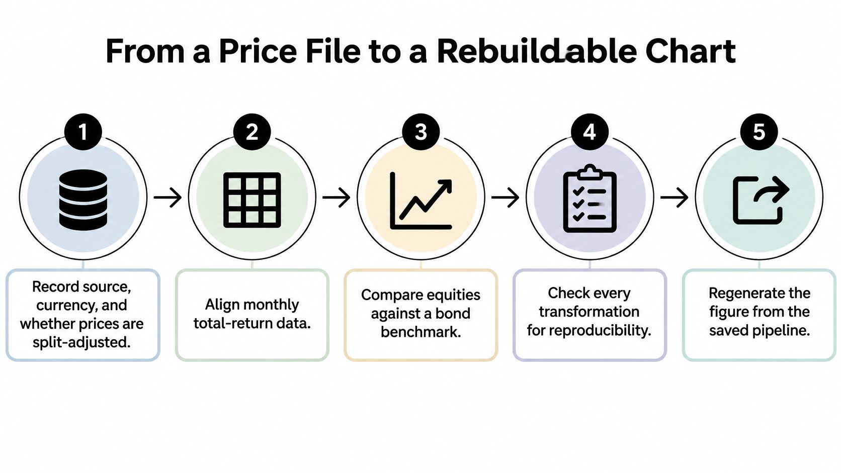
Build the analysis in a reproducible sequence
Record provenance and meaning. Save the source, retrieval information, currency, field definitions, and adjustment status. Split adjustment alone doesn't establish total return: verify how dividends, distributions, and reinvestment are represented.
Align both series to a common monthly calendar. Count missing periods before filling anything, and inspect the underlying session coverage if daily inputs are available. Don't carry forward a missing value, because that can create an artificial flat return.
Choose the return definition. Simple returns suit wealth accumulation through compounding. Log returns suit additive time aggregation for positive values, but they aren't interchangeable with simple returns in a portfolio calculation. Write down which definition answers the question.
Create a cumulative-return line and a separate drawdown panel. Calculate drawdown relative to the running peak, and retain the same date alignment in both panels. This separates where wealth finished from the path investors experienced.
Add a defined comparison range. If the question concerns the mean equity-minus-bond return, show its estimation interval in a companion panel. If the question concerns realized dispersion, label a historical outcome range instead. Don't shade arbitrary space around a cumulative curve and call it uncertainty.
Add only a couple of dated events that materially affect interpretation. Obtain their dates from documented records, and distinguish source corrections from economic events.
Publish a companion table. Include start date, end date, cumulative return, maximum drawdown, and sample size for each series. Explain exclusions and distinguish the number of price observations from the number of computed returns.
Save the source file, transformation code, environment information, chart settings, and output table. Rebuild the figure from a clean session rather than from objects left in memory.
Keep the code sketch honest
In pandas, sort the dated total-return index and use pct_change(fill_method=None) for simple periodic returns. Compound valid returns into cumulative performance, plot the result in percent, and use Matplotlib's fill_between only with lower and upper limits calculated by a documented method.
That's a visualization pipeline, not a complete backtest. It doesn't establish execution timing, transaction costs, investability, or out-of-sample predictive performance.
The same distinction matters in operating forecasts. Jumpstart Partners' guide to forecast SaaS revenue and expenses offers a related modeling context: assumptions and transformations must remain inspectable alongside the resulting chart.
Preserve machine-readable meaning
For issuer comparisons, the SEC financial-statement datasets provide flattened, XBRL filing-derived face-statement numbers. Preserve concept tags, fiscal periods, units, currencies, and dimensional qualifiers; standardized extraction doesn't guarantee that superficially similar metrics are economically equivalent.
Keep public survey charts tied to their question definitions, too: the FCA Financial Lives survey had 17,950 respondents in 2024. The denominator for a particular chart may be a relevant subgroup rather than every respondent.
Use stable field names, a data dictionary, and machine-readable exports so another script can join and regenerate the records. Keep account-level holdings on a machine the analyst controls, and aggregate shared outputs carefully enough that readers can't reconstruct sensitive positions from labels, totals, or small groups.
Chart Pitfalls That Distort Returns and Risk
An interactive chart isn't automatically a validated chart. A University of Arizona experiment involving 157 participants found that visualization or interactivity alone worsened calibration, while their combination improved confidence and accuracy.
The practical implication is narrower than “add more interaction.” A filter or zoom needs a stated check: what evidence should the user inspect, and how will they know whether their conclusion is justified?
Review the claim after the figure exists
| Symptom | How it misleads | Fix |
|---|---|---|
| Two series on dual axes | Aligned slopes imply a false link | Split the series into separate panels |
| Bars with a cut axis | A small gap looks large | Start amount bars at zero |
| Pie, bubble, or 3D volume | Angle and volume hide close values | Use a ranked dot plot |
| Red cell with no threshold | Hue feels like a larger loss | Show the delta, baseline, and cutoff |
| Interactive filter only | Confidence rises faster than accuracy | Pair interaction with a stated check |
| Correlation heatmap as a story | Association is read as cause | Print coefficients and refuse a causal caption |
| Equity curve of survivors | Compounding is overstated | State the universe, lags, and dropped names |
| Ranked gaps inside overlapping intervals | An unresolved difference looks decisive | Withhold the ranking unless a direct comparison supports it |
Presentation affects interpretation even when the records don't change. A financial-risk communication study involving 40 participants found that graphics helped users compare patterns, written explanations supported precise interpretation, and red elements were treated as stronger warnings.
Likewise, a 2021 Cognitive Fit experiment with 95 accounting undergraduates linked presentation format to the speed of detecting potentially fraudulent transactions from identical information. That supports matching format to task, not assuming every visual display improves every decision.
Separate exploration from confirmation
An anomaly scan identifies records worth investigating. It doesn't establish fraud, causality, or a repeatable investment opportunity.
For a candidate signal, check whether the universe includes failed or delisted entities and whether every input was available when the decision would have occurred. If you searched many relationships, disclose that exploration and use appropriate validation rather than presenting the strongest-looking result as a prespecified finding.
Overlapping marginal intervals also don't settle the uncertainty of a difference. Estimate the contrast directly, accounting for paired observations or dependence when relevant.
A final data visualization best-practices review should inspect the numerical claim, not merely typography and spacing. Ask whether the reader could reach a different conclusion after learning what was excluded.
Choose a Tool That Can Rebuild the Figure
| Tool | Best for | Code and method visibility | Limit |
|---|---|---|---|
| PlotStudio AI | Multi-step investigation of a return file | Inspectable Python and a saved Analysis Page | The analyst still must set the question and definition |
| Hand-written notebook | Full manual control under existing review | Every line is the author's | Manual profiling, documentation, and reruns require maintenance |
| Chat-with-data tool | One-off sketch of public data | Check whether code and a persistent method are available | Cleaning and the audit trail can be skipped unless explicitly preserved |
Choose among AI tools for data analysis by the evidence they preserve. A hand-written notebook may fit an established code-review process best. A conversational interface can be sufficient for a disposable public-data sketch, provided you don't mistake the sketch for a reproducible analysis.
Where agentic analytics fits
Agentic analytics is data analysis performed by AI agents that can plan an investigation, execute analytical steps with real tools and code, inspect intermediate results, revise the approach, validate outputs, and synthesize a complete analysis. An answer is an output; an analysis is an investigation.
PlotStudio AI is an AI tool for researchers who need to investigate data, not merely chat with it. Its workflow supports uploading a return file, reviewing a plan, executing Python locally, inspecting intermediate outputs, and saving a permanent Analysis Page containing tables, charts, statistical tests, and interpretation. Domain methods include GARCH volatility models, RSI, MACD, and Bollinger Bands; other domains include clinical survival curves, FDR correction across 20K genes, and spatial autocorrelation. Exports include a one-click PDF with charts, formatted tables, and rendered LaTeX, plus a Jupyter notebook containing code and outputs.
PlotStudio AI didn't invent agentic analytics. It can be considered a Julius AI alternative for researchers prioritizing multi-step investigation, local Python execution, methodology visibility, and reproducibility.
For broader selection criteria, compare data visualization software. The Effortless Academic review offers an independent product assessment, while the HeliosNet market research blog is a separate source of market-oriented reading, not validation of a chart's calculations.
Common questions
What's the best chart for financial data?
Choose the chart from the decision: paths, cross-sectional comparisons, distributions, and forecasts need different encodings.
Can AI validate a finance chart?
AI can execute checks, but researchers must judge definitions, assumptions, comparability, and decision relevance.
What makes a financial chart reproducible?
Preserved inputs, documented transformations, executable code, and enough metadata to regenerate the figure.
An honest figure lets another researcher inspect both the conclusion and the route used to reach it. That's a stronger selection criterion than appearance alone.
Download and try PlotStudio AI with a non-sensitive return file and a clearly defined comparison. New researcher accounts include 1,000 free credits while the offer is active.