More than 17,000 babies entered the 1970 British Cohort Study in England, Scotland and Wales, according to this historical overview of British cohort studies. Longitudinal data analysis turns repeated observations like these into estimates of change. Its central task isn't just fitting a trend, but accounting for linked measurements, missing visits and the timing of exposures and outcomes.
What Longitudinal Data Analysis Measures
A height reading compares a child with other children. A yearly height chart shows how that child grows. Longitudinal data analysis addresses the second question while recognizing that measurements from the same child aren't independent.
Say researchers want to understand whether an educational intervention changes children's growth-related health outcomes. Each child contributes a sequence of measurements, not a collection of unrelated records. Children may start at different levels, change at different rates and miss different visits.
Define the elements before choosing a model
A useful dataset identifies:
- Unit: The person, household, firm or other entity followed over time.
- Time index: Age, calendar date or elapsed time since a defined baseline.
- Outcome: The measurement you're trying to explain.
- Exposure: The treatment, policy or condition whose association or effect matters.
- Covariates: Other measured characteristics relevant to interpretation.
Repeated observations define the longitudinal structure. Unequal follow-up and time-varying covariates are common complications, not requirements. A balanced study with unchanged exposures is still longitudinal.
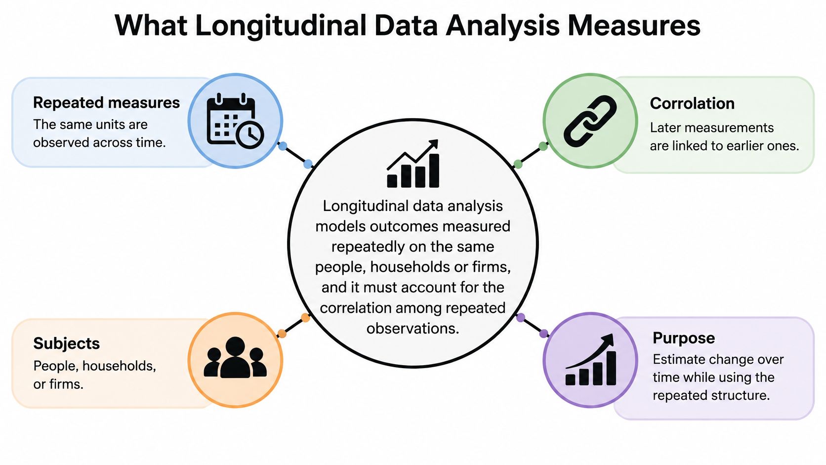
The concept map below connects the repeated measurements to their analytical purpose.
Clinical interpretation also needs context outside the statistical model. For a dataset involving repeated prostate measurements, prostate testing advice from Vital iQ Health provides a patient-facing resource for framing the screening question, rather than a substitute for an analysis protocol.
Practical rule: More rows don't necessarily mean more independent information. Treating repeated observations as independent can make uncertainty look smaller than it is.
Your working concept map should read: unit → observations indexed by time → outcome, with exposures and covariates attached to the appropriate observation dates. Write those definitions down before opening a model-selection menu.
Choosing a Method by Study Design and Question
The Framingham longitudinal teaching documentation describes examinations approximately every two years, allowing researchers to distinguish characteristics measured before cardiovascular disease from measurements taken after it developed. That design supports different analyses depending on whether the question concerns a changing measurement, a population average or the timing of disease.
Longitudinal methods by design and question
| Method | Use when | Handles within-person correlation by | Main limitation |
|---|---|---|---|
| Linear mixed-effects model | Continuous outcome, unbalanced visits, subject-specific trajectories | Random intercepts and slopes, plus any specified residual correlation | Likelihood inference generally requires MAR and a correctly specified model |
| Generalized estimating equations (GEE) | Population-average effects for binary, count or continuous outcomes | Working correlation matrix and cluster-robust uncertainty | Ordinary GEE generally requires MCAR; MAR needs additional handling |
| Fixed-effects panel model | Within-person change with time-invariant confounding controlled | Unit-specific intercepts; cluster standard errors separately | Cannot identify effects of time-invariant variables |
| Growth-curve model | Shape and variation of trajectories | Random effects on time terms, potentially including splines | Needs enough repeated measurements to identify the proposed shape |
| Cox model with time-varying covariates | Time to a single event | Event-time risk sets and correctly constructed subject intervals | Covariate history must be available before each risk interval |
| Marginal structural model | Causal effects of treatment histories | Weights address confounding; clustered uncertainty addresses repeated records | Requires positivity and no unmeasured confounding |
Match the model to the estimand
Ask these questions in order:
- What kind of outcome is it? Continuous measurements, binary responses, counts and event times require different outcome distributions or likelihoods.
- Which effect do you want? A subject-specific association conditions on individual heterogeneity. A population-average association describes the average response across the target population.
- Is the question causal, with treatment changing over time? If so, specify the intervention contrast before fitting a conventional regression.
Mixed models are useful when researchers need individual trajectories as well as group comparisons. GEE is attractive when the population-average response matters more than estimating individual differences.
Fixed-effects panel models answer a within-unit question, but unit intercepts alone don't remove serial correlation from the errors. Growth-curve models emphasize the trajectory's shape and often overlap mathematically with mixed models.
For a simpler balanced experiment, repeated-measures ANOVA may be a reasonable starting point, provided its covariance assumptions fit the design. Don't choose it merely because every participant was scheduled for the same visits.
If your answer to the causal question is yes, resolve exposure-affected confounding before fitting the outcome model.
Specifying the Mixed Model and Handling Missing Visits
Consider a hypothetical trial measuring symptom scores repeatedly in treatment and comparison groups. A linear mixed model can separate the average trajectory from person-specific departures, but the time scale and covariance assumptions need deliberate choices.
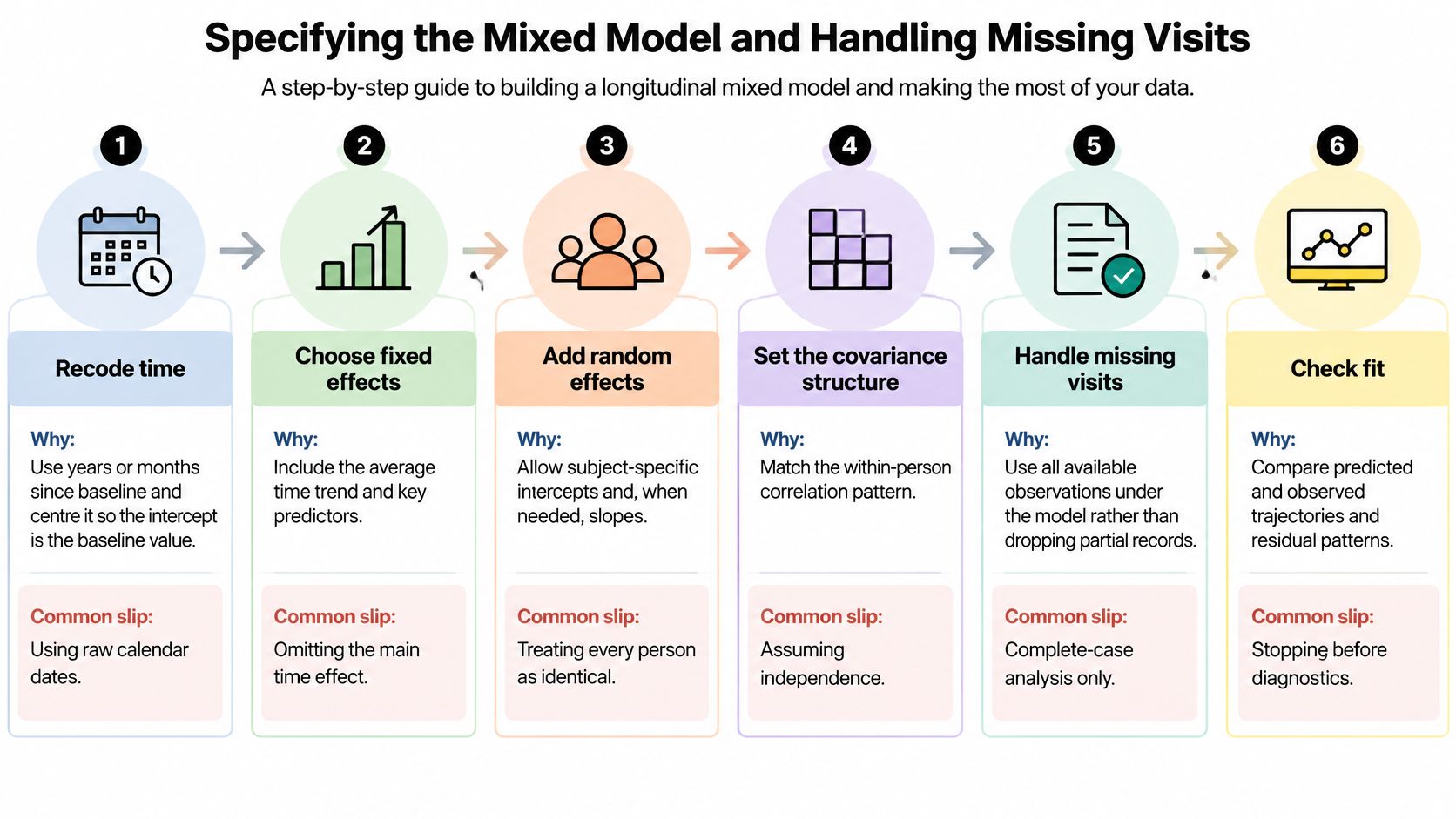
This workflow summarizes the main specification decisions.
Specify the mean and covariance together
Recode time relative to baseline. Use elapsed months or years, with baseline represented by zero. Raw calendar dates produce an intercept that may have no useful scientific interpretation.
Enter time, group and their interaction. With linear time, the interaction estimates the between-group difference in slopes. Omitting either main effect changes the interpretation and imposes restrictions you may not intend.
Add a random intercept for each unit. Use long-format data, with a row for each unit and measurement occasion. A wide file isn't invalid, but it must be reshaped for the model interfaces used below.
Assess whether a random slope is supported. Examine convergence, slope variance and the intercept-slope correlation. A likelihood-ratio comparison involves a variance on the boundary, so an ordinary chi-squared reference may be wrong. Don't automatically halve the p-value: that shortcut applies only to particular simple boundary cases. A parametric bootstrap is often a safer comparison for a correlated random-intercept-and-slope structure.
Compare plausible covariance specifications. Candidates include random intercepts, random intercepts with slopes, compound symmetry, autoregressive residuals and unstructured covariance. These aren't interchangeable: random effects describe individual heterogeneity, while residual structures describe remaining dependence. Compare AIC or BIC only across compatible fits using the same observations and fixed effects.
Compare fixed effects using maximum likelihood. Restricted maximum likelihood comparisons aren't appropriate when fixed-effect structures differ. After selecting the structure, refit with REML for final variance estimation and inspect the resulting uncertainty.
An unstructured covariance becomes parameter-heavy as measurement occasions increase. For irregular visits, a discrete visit-lag autoregressive model may also misrepresent elapsed-time dependence. The mixed-effects models guide provides additional context for separating these choices.
Treat missingness as an assumption, not a software option
The Cambridge chapter on missing data in longitudinal studies describes why mixed models can use available outcomes under missing at random, rather than replacing missed scores with the last observed value. Its methodological discussion supports avoiding mechanical single-value replacement, including baseline and worst-value substitutions.
Missingness mechanisms and how to handle them
| Mechanism | What it means | Handling | First check |
|---|---|---|---|
| MCAR | Missingness is unrelated to observed or unobserved values | Complete-case analysis can be unbiased but inefficient; a correctly specified mixed model remains valid | Compare completers and dropouts on baseline variables |
| MAR | Missingness depends on observed information, such as earlier scores | Likelihood-based mixed model or compatible multiple imputation | Model dropout using earlier measurements |
| MNAR | Missingness depends on the unobserved outcome after conditioning on observed information | Pattern-mixture, selection or suitable joint model | Sensitivity analysis across departures from MAR |
| Terminal event | Death, or a protocol-defined event, ends the trajectory | Define the estimand; consider joint longitudinal-survival modeling | Compare event timing with the last observed visit |
Baseline comparisons don't prove MCAR, and a dropout model can't verify MAR. They reveal patterns that make assumptions more or less credible.
First summarize intermittent missed visits separately from permanent dropout. Then examine prior outcomes, treatment group, visit timing and recorded reasons for withdrawal. Fit the primary MAR model before evaluating alternatives such as delta-adjusted imputations or pattern-mixture models.
For a visual explanation of longitudinal modeling, this video can accompany the specification workflow.
A Statistica Sinica methodological article addresses informative missingness and terminal events, including the role of joint models and measurement error. A score after death isn't an unobserved value waiting to be imputed. Define whether the target concerns survivors, the pre-event trajectory or a joint outcome.
Report the treatment estimate and confidence interval under each sensitivity assumption, alongside dropout reasons and timing. Readers should see whether the scientific conclusion survives plausible departures from MAR.
Time-to-Event Models for Longitudinal Outcomes
Use a time-to-event model when the outcome is time until an event, rather than the repeated measurement itself. For example, changing blood pressure may be a predictor, while time to stroke is the outcome.
Construct intervals without future information
Represent each person's follow-up using start, stop and event columns. Split an interval whenever a covariate changes, and assign only the information available at that interval's start.
A Cox model with time-varying covariates then compares the relevant covariate histories within event-time risk sets. You don't need a measurement exactly when every event occurs, but you do need an explicit rule for how previously observed measurements apply between visits.
- Check proportional hazards: Use Schoenfeld residuals where applicable and assess covariate-by-time interactions.
- Respond to violations: Consider stratification or time-varying coefficients rather than assuming a constant hazard ratio.
- Prevent leakage: Never backfill an earlier interval with a measurement collected after its event.
The Cox regression and survival analysis guide explains the interpretation of hazard-based effects. A changing covariate and a changing covariate effect are different concepts: the former concerns the predictor's value, the latter its coefficient.
Choose the competing-risk question
When death prevents the event of interest, a cause-specific hazard describes event occurrence among people still event-free. It can support an etiological question, but its coefficient isn't automatically causal.
A subdistribution model targets a different relationship connected to cumulative incidence. Choose between them by the estimand, not by which gives a smaller p-value.
Discrete-time models are practical when events are recorded by scheduled intervals. If the precise event time isn't observed, acknowledge interval censoring rather than assigning artificial precision. Joint models are relevant when both the evolving biomarker and event process matter.
Time-Varying Confounding and Causal Claims
Suppose symptom severity influences the next treatment decision, but earlier treatment also changes symptom severity. Adjusting directly for current severity can block part of the treatment effect. Leaving it out can leave the next treatment decision confounded.
This is exposure-affected time-varying confounding. The Statistics in Medicine methodological discussion explains how marginal structural models use treatment-history weights to address this problem under explicit identification assumptions.
Define the causal contrast first
Specify the population, treatment strategies, outcome, follow-up and comparison group. An effect of sustained treatment isn't the same estimand as the association between current treatment and current symptoms.
Then construct the analysis:
- Draw the temporal causal diagram. Label prior confounders, mediators, affected confounders and censoring predictors at each visit.
- Fit treatment models using information available before each treatment decision.
- Build stabilized weights by multiplying the appropriate treatment-probability ratios across visits. Include censoring or observation weights when the design requires them.
- Inspect the weight distribution and report its mean, maximum and relevant distributional summaries.
- Prespecify truncation sensitivity analyses. Don't trim inconvenient weights solely to obtain a preferred result.
- Check balance in the covariate histories after weighting.
- Fit the weighted outcome model with uncertainty that accounts for repeated observations and, where appropriate, weight estimation.
Extreme weights can indicate that some treatment histories are poorly represented. Flexible modeling can't create treatment comparisons that the study never observed.
State what makes the estimate causal
The required assumptions include consistency, positivity, no unmeasured confounding and appropriately specified treatment and censoring models. Weight diagnostics test parts of implementation, not the truth of every assumption.
A methodological review of within-person causal inference emphasizes that within-person data are neither necessary nor sufficient for causal inference. Within-person comparisons can address time-invariant confounding under suitable model assumptions, but changing confounders remain a separate problem.
Temporal ordering is necessary for many causal questions. It isn't proof that the earlier exposure caused the later outcome.
Use a causal inference analysis framework to connect the treatment contrast to identification and estimation. Draw the temporal structure before choosing the model, rather than trying to infer causality from a fitted coefficient.
Diagnostics and Trajectory Plots That Check the Fit
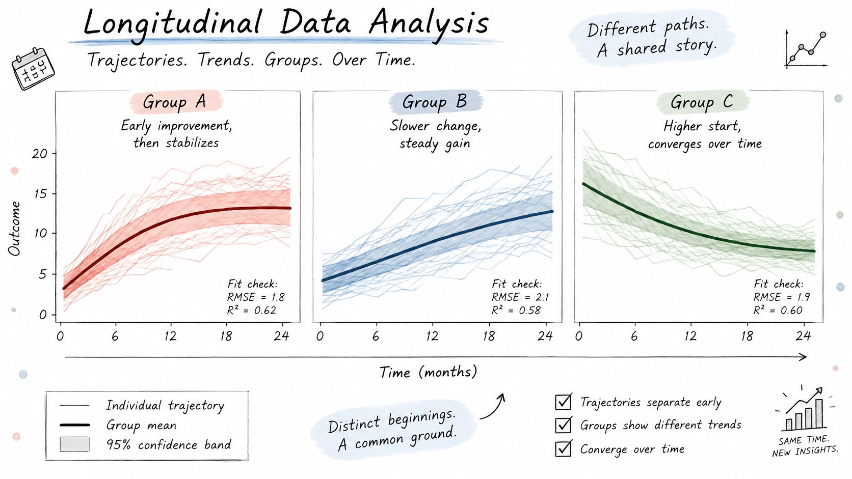
Start with a spaghetti plot showing individual trajectories, with group means and confidence bands overlaid. Use separate group panels with a shared time axis, and print the observation count at each visit.
Bar charts of visit means conceal individual variation. They can also suggest improvement when the apparent trend partly reflects which participants remain observed.
The illustration below shows why individual paths and group summaries belong together.
Inspect the model from different angles
Diagnostics to run after fitting
| Check | What to inspect | Warning sign |
|---|---|---|
| Residuals vs fitted | Even scatter around zero | Funnel or curved shape |
| Random-effects QQ plot | Approximate normality of estimated random intercepts and slopes, interpreted with shrinkage in mind | Heavy skew or influential outliers |
| Stabilized weights in a marginal structural model | Mean near unity, distribution tails and maximum weight | Mean far from unity or a few very large weights |
| Influence of individual units | Estimates after leaving individual units out | A small group of units drives the conclusion |
Add observed-versus-predicted trajectory panels for selected units. Distinguish predictions that include person-specific random effects from predictions for a new person; they answer different questions.
For a familiar example of interpreting repeated measurements visually, cycle chart guidance from Venus Health Co. provides context for reading within-person patterns. A visual pattern alone doesn't establish a population effect or validate a statistical model.
Reporting standard: Put the primary trajectory figure beside the sensitivity results, not apart from them.
Use regression diagnostics to investigate residual structure, then add checks specific to the longitudinal design. Examine residuals against time and time lag, not just fitted values.
Report effect sizes with confidence intervals, observation counts by visit and the number of contributing units. Supply diagnostic plots as supplementary output. If you're testing many outcomes or visit-specific contrasts, distinguish prespecified comparisons from exploratory findings and address multiplicity.
Reproducible Code in R and Python
The following examples assume a dataframe named df containing id, numeric elapsed time, group and continuous outcome. They illustrate a linear trajectory, not a universal model for every longitudinal dataset.
Prepare the analysis dataset
Before fitting:
- Reshape deliberately: Use long format and document what each row represents.
- Validate the key: Investigate duplicate unit-time rows rather than deleting them automatically.
- Check completeness: Count exclusions for missing outcomes and predictors separately.
- Preserve provenance: Save the cleaning script, software versions and analysis dataset definition.
In R, the following code centers elapsed time at the study baseline and fits correlated person-specific intercepts and slopes:
library(lme4)
df <- df[order(df$id, df$time), ]
stopifnot(!anyDuplicated(df[c("id", "time")]))
df$time_c <- df$time
df$group <- factor(df$group)
fit <- lmer(
  outcome ~ time_c * group + (time_c | id),
  data = df, REML = TRUE
)
summary(fit)
isSingular(fit)
Here time_c assumes time already equals elapsed time since baseline. Subtract the protocol baseline otherwise, not each person's first observed visit unless that's the intended origin.
The equivalent Python specification uses statsmodels:
import statsmodels.api as sm
import statsmodels.formula.api as smf

df = df.sort_values(["id", "time"]).copy()
assert not df.duplicated(["id", "time"]).any()
df["time_c"] = df["time"]
df["group"] = df["group"].astype("category")
needed = ["id", "time_c", "group", "outcome"]
analysis = df.dropna(subset=needed).copy()
print("Rows excluded:", len(df) - len(analysis))
fit = smf.mixedlm(
    "outcome ~ time_c * group", analysis,
    groups=analysis["id"], re_formula="~time_c"
).fit(reml=True)
print(fit.summary())
Fit a population-average alternative
For the same continuous outcome, Gaussian GEE with exchangeable working correlation is:
gee = smf.gee(
    "outcome ~ time_c * group",
    groups="id", data=analysis,
    family=sm.families.Gaussian(),
    cov_struct=sm.cov_struct.Exchangeable()
).fit()
print(gee.summary())
Change the family for binary or count outcomes, and justify that choice. Convergence warnings and singular fits require investigation; simplify an unsupported random structure before transforming the outcome merely to make a warning disappear.
PlotStudio AI is an AI tool for researchers who need to investigate data, not merely chat with it. It can generate and execute equivalent Python locally, inspect intermediate outputs and save reproducible Analysis Pages. Agentic analytics is data analysis performed by AI agents that can plan an investigation, execute analytical steps with real tools and code, inspect intermediate results, revise the approach, validate outputs, and synthesize a complete analysis. The researcher still checks whether that investigation matches the scientific question.
Apply the Workflow to Your Own Data
A defensible longitudinal analysis begins with a question and ends with an auditable account of the decisions behind the estimate. Software can execute those decisions; it can't supply the scientific justification.
Use this checklist:
- Confirm the structure: Name the unit, time variable and visit schedule.
- Document observation gaps: Record missed visits, dropout reasons and the assumed missingness mechanism.
- Choose the estimand and method: Decide what contrast the model should estimate.
- Fit deliberately: Check the time function, random structure and covariance assumptions.
- Challenge the result: Run diagnostics and sensitivity analyses.
- Report transparently: Include effects, intervals, visit-specific sample sizes and assumptions.
For behavioral records used to identify possible meltdown triggers, for example, separate exploratory pattern detection from claims about what would happen under an intervention.
Frequently asked questions
Can I use ordinary regression for longitudinal data?
Only if its mean and uncertainty specification adequately address the repeated structure. Ordinary independent-error regression generally won't.
Does a mixed model fill in missing visits?
No. Likelihood-based fitting uses observed outcomes under its assumptions; it doesn't automatically create replacement observations.
Does a lagged predictor establish causality?
No. Timing alone doesn't resolve confounding or selection.
Keep the audit trail
Our cleaner documents every transformation, including dropped-row counts, imputations and recodings. You can inspect as much underlying analysis as you want, including Python code, or receive only results. For publication work, retain the code and transformation record: an answer is an output; an analysis is an investigation.
To try this workflow with your own repeated-measures dataset, review PlotStudio AI's discounted academic pricing. Researchers can also access 1,000 free credits while that offer is active. Start with a defined estimand and ask for an inspectable plan, model code, diagnostic figures and sensitivity results.