Omitted variable bias is the systematic error a regression coefficient absorbs when a factor that affects the outcome also moves with an included regressor and gets left out of the model. It survives any sample size, and it leaves no footprint in your output. The popular fix, adding more controls, doesn't solve it. Knowing the direction of the bias and the strength a confounder needs to overturn your conclusion does.
The advice to control for everything is the most popular remedy in applied work and among the least reliable. A control you can't place on a causal graph moves the coefficient without telling you why, and a noisy proxy can leave you carrying two biases where you had one.
The Sign of Omitted Variable Bias
Write down two models before you estimate anything. The long model is the one the world obeys. The short model is the one you can fit, because one regressor is missing from your data. Omitted variable bias is the gap between what the short model converges to and the long model's true coefficient.
In symbols, with X as your regressor of interest and Z as the factor you left out, the short-model estimator converges to
plim(b̂) = βx + βz · δ
where βz is the omitted factor's true effect on the outcome and δ is the slope from the auxiliary regression of Z on X, holding the other included regressors fixed. That single expression is the formula you'll reuse in every model you fit.
Where the second term comes from
Four lines get you there.
- Write the true model as Y = βx X + βz Z + error.
- Project the omitted factor on what you did include, Z = δ X + v, with v uncorrelated with X once the other controls are partialled out.
- Substitute to get Y = (βx + βz δ) X + βz v + error.
- The short regression therefore converges to βx + βz δ, not to βx.
Nothing in that derivation assumes a small sample. The bias is a property of the probability limit, so more data makes the estimate more precisely wrong rather than less wrong.
Reading the four cells with wages
Take the canonical example: wages regressed on years of schooling, with ability omitted. Ability raises wages, so βz = 0.40. People with more ability also tend to stay in school, so the auxiliary slope is δ ≈ 0.50. Multiply and the short regression overstates the return to schooling by 0.20.
| Case | Effect of Z on Y | Association of Z with X | Bias in the X coefficient |
|---|---|---|---|
| Z raises Y and moves with X | Positive | Positive | Away from zero if the true effect is positive; coefficient biased upward |
| Z raises Y and moves against X | Positive | Negative | Coefficient biased downward |
| Z lowers Y and moves with X | Negative | Positive | Coefficient biased downward |
| Z lowers Y and moves against X | Negative | Negative | Coefficient biased upward |
The two signs do all the work. An omitted factor that raises the outcome and moves with your regressor pushes the coefficient away from zero. An omitted factor that raises the outcome but moves against your regressor pulls it toward zero. Flip either sign and the direction of the bias flips with it.
Practical rule: before you open a robustness table, record the sign you expect for βz and the sign you expect for δ. If the coefficient moves the other way, your story about what was omitted is wrong.
Three confusions are worth clearing up. First, this is inconsistency, not imprecision: the standard error can shrink while the center of the distribution stays wrong, so a tight interval around a biased estimate is worse than a wide one. Second, R² can rise when you add a control while the causal coefficient gets worse, because fit and identification answer different questions. Third, adding an irrelevant regressor inflates variance but doesn't create this bias, since the formula needs both terms to be nonzero.
Conditioning on a collider produces a different bias with different algebra, so the formula doesn't cover it. That distinction is the next thing to get straight.
Back-Door Paths That Match the Formula
An arrow diagram isn't decoration. It's the shortest statement of which variables cause which, and it's where both terms in the formula come from.
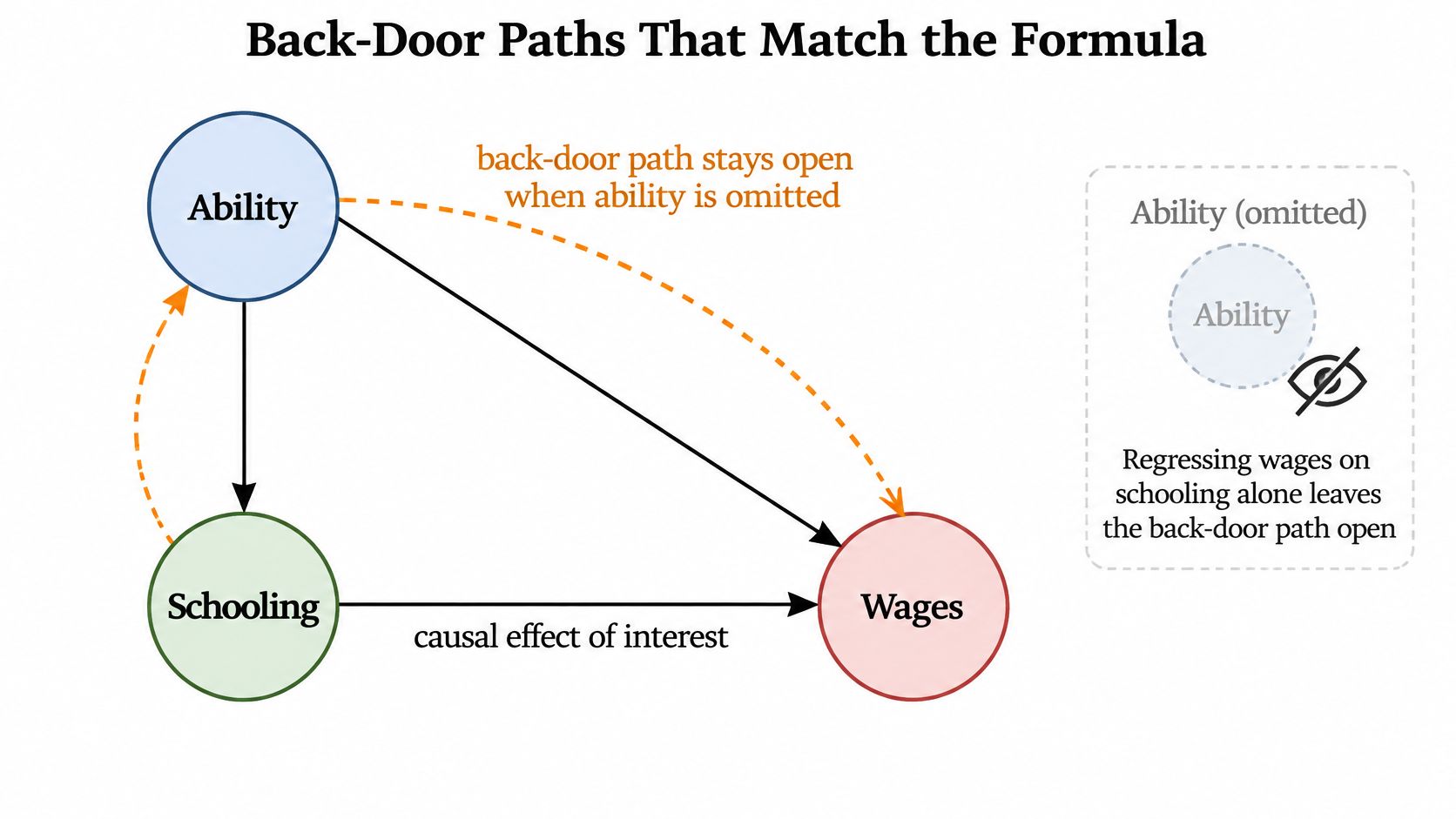
For the wage case the graph has three nodes. Ability points to schooling and to wages, and schooling points to wages. The last arrow is the causal effect you're after. The other two form a back-door path, Schooling ← Ability → Wages, and it stays open as long as ability sits unobserved in the error term.
The diagram below draws that graph and marks the path that never closes.
Two arrows, two terms in the formula
The arrow from ability to wages is βz: it sets how much the omitted factor matters for the outcome. The arrow from ability to schooling is why δ isn't zero: it's the reason the omitted factor and your regressor travel together.
Both arrows must exist for bias to appear. A factor with a strong arrow into wages but no relationship to schooling lands in the error term and stays uncorrelated with your regressor. That omission costs you a little precision and nothing else.
The back-door criterion is worth memorizing as one sentence: a valid control set blocks every open back-door path, leaves every causal path open, and conditions on no collider. Control selection follows from that and from nothing else.
Two graphs that look like fixes and aren't
Occupation as a mediator. Schooling changes occupation, and occupation changes wages. Occupation sits on the causal path, not on a back door. Add it and you stop estimating the total return to schooling; you estimate the piece that doesn't run through occupation. The coefficient moves because the estimand changed.
Sample selection as a collider. Suppose the sample includes only people who both finished school and hold a job, so selection is caused by schooling and by wages. Conditioning on selection opens a path that was closed. A coefficient that shifts when you restrict the sample may be manufacturing a problem rather than revealing one.
A control is a claim about the world, not a checkbox in a dataset. If you can't draw the arrow, you can't defend the adjustment.
The graph is an argument you have to make, not a picture of whichever columns happen to be in the file. That's the same discipline described in Thesis Book Project's explainer on what a theoretical framework is in research: the framework is the claim, and the data is evidence brought to bear on it rather than a substitute for it.
If you want the wider menu of designs that follow from a graph, this guide to causal inference analysis works through identification strategies rather than control lists.
The practical translation is blunt. If you can't name the open back-door path, you can't say which sign the bias should have, and a coefficient's movement can't be used as evidence of anything.
A Schooling Estimate That Moves by 0.20
Predictions about sign are cheap to state and hard to believe until you watch a number move. So generate a dataset where you already know the answer.
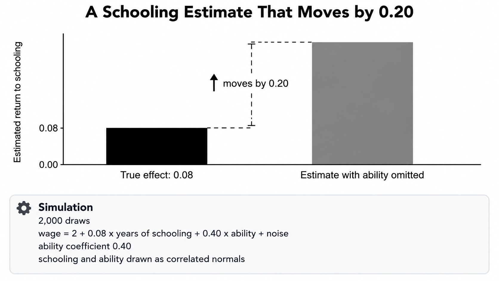
Set the true equation to wage = 2 + 0.08 × years of schooling + 0.40 × ability + noise, draw 2,000 observations, and let schooling and ability be correlated normals with a correlation near 0.5 and similar spread. Because the two regressors share that correlation, the auxiliary regression of ability on schooling returns a slope δ ≈ 0.50, and the formula predicts a bias of 0.40 × 0.50 = 0.20.
Here is what that shift looks like against the true effect.
Three fits on the same draws
Fit the long model and the schooling coefficient comes back near 0.08. Drop ability and it climbs to about 0.28, which is the 0.20 the algebra promised. Then try a common move: build a proxy equal to ability plus classical measurement error and put that in the model instead. The coefficient lands near 0.22. Better than 0.28, nowhere near 0.08.
| Model | Schooling coefficient | What it shows |
|---|---|---|
| Full model with ability | 0.08 | Recovers the true return |
| Ability omitted | 0.28 | Overstates the return by the predicted 0.20 |
| Noisy proxy equal to ability plus classical error | 0.22 | Imperfect proxy does not close the gap |
| Auxiliary regression of ability on schooling | δ about 0.50 | Supplies the multiplier for the 0.40 ability coefficient |
The proxy stalls because its own noise attenuates its coefficient, so part of ability's effect stays loaded onto schooling. The auxiliary regression is what makes the whole check verifiable: regress ability on schooling, read the slope, multiply by the ability coefficient you believe in, and compare that product to the gap between your short and long estimates.
Enough code to regenerate it
Four steps, no more.
- Draw schooling from a normal, then draw ability as a correlated normal with
np.random.multivariate_normalso the correlation is set explicitly rather than inherited. - Build wages from the linear combination plus
np.random.normalnoise, and stack everything in a DataFrame. - Fit
sm.OLS(y, sm.add_constant(X)).fit()three times: with ability, without it, and with the error-laden proxy. - Print
.paramsbeside the auxiliary regression and check whether 0.40 × δ matches the observed gap.
The walkthrough below covers the same logic in more depth.
What the 0.20 does and doesn't settle
These are illustrative population draws, not a published labor-market estimate, and a real analysis should put a confidence interval next to the point shift rather than reporting the shift alone. With 2,000 observations each interval is narrow enough that the gap isn't sampling noise, which is the uncomfortable part: the estimate is precise and wrong.
The decision test isn't whether the omitted term is nonzero. It's whether a 0.20 move changes the claim you want to make. A paper arguing that schooling returns are positive survives a shift from 0.08 to 0.28, because the sign holds. A policy memo arguing the return clears a stated threshold doesn't survive it, because threshold claims and sign claims fail differently under the same bias.
The same reasoning applies when your regressor isn't something you assigned. Estimating an effect on the treated instead of an average effect changes which comparison is contaminated, so it's worth knowing how that estimand is defined before you read a movement as bias rather than as a different question.
Checks That Are Not Just More Controls
A coefficient that jumps when you add a covariate feels like proof of something. It isn't. Movement is consistent with confounding, with a changed estimand, and with ordinary sampling variation, and the output looks the same in all three cases.
What each diagnostic actually tests
Residual plots and a Ramsey RESET speak to functional form. Curvature in the residuals means the linear specification is wrong, which can push a coefficient in either direction with no omitted variable involved.
Variance inflation factors describe collinearity among regressors already in the model. High VIFs widen intervals; they don't bias a coefficient. Confusing the two sends people hunting for dropped variables when the problem is that two included variables measure nearly the same thing.
A coefficient difference across subgroups can be real heterogeneity in the effect rather than a forgotten control. Before you call it bias, ask whether the effect itself could plausibly differ by group, because if it can, forcing one coefficient across groups is the specification error.
Fit criteria make things worse rather than better. Link tests and information criteria will happily prefer a model with better prediction while the back-door path stays wide open.
A five-step check you can run in an afternoon
- Name the omitted factor on the graph. If it isn't a node with arrows, you have a hunch rather than a bias story.
- Predict the sign of βz × δ. Write it down before you look at the long model.
- Compare short and long estimates. Check the sign of the gap and its rough size against the prediction.
- Reject bad controls. A mediator or collider that moves the coefficient is a reason to drop it, not keep it.
- Escalate if the gap survives. A large unexplained gap is an identification problem, and no chart resolves it.
A specification curve is useful here if you read it correctly. It maps how the estimate depends on defensible choices, and a flat curve is reassuring. It's not proof that your preferred point is causal, because every point on the curve can share the same unmeasured confounder.
A table full of controls is evidence that you ran more regressions, not evidence that you identified anything.
When the confounder is real and unmeasured, the honest move is a design change. That usually means an instrument or a panel, and the mechanics matter: this guide to instrumental variable regression covers relevance, exclusion, and the weak-instrument failure mode.
Controls, Fixed Effects, and Instruments
Every remedy leans on a different slice of variation, and each fails in a specific way. The table is the map. The rest of this section is about the row people misread.
| Approach | What it can remove | What it requires | When it fails |
|---|---|---|---|
| Additional controls | Measured confounders on open back-door paths | Correct functional form and no bad controls | Colliders, mediators, or a still-unmeasured factor |
| Fixed effects or first differences | Unobserved factors fixed within the panel unit | Panel data and within-unit variation in treatment | Time-varying confounders or no within variation |
| IV or 2SLS | Endogeneity from omitted factors correlated with X | A relevant instrument that affects Y only through X | Weak instruments or exclusion failure |
| Placebo or negative control | Nothing by itself; it detects a leftover association | An outcome or sample that should be null | A real effect on the placebo, or a placebo that is not comparable |
Matching the remedy to the variation
Additional controls work when the confounder is measured, the functional form is roughly right, and the new variable sits on a back door rather than a causal path. That's a narrow set of conditions, and it's the set people skip.
Fixed effects absorb anything constant within a person, firm, region, or other panel unit. That's a strong claim to be able to make, because plenty of confounding doesn't change over the observation window. The price is that you need within-unit variation in the treatment, and time-varying confounders survive untouched.
Instruments swap the contaminated part of X for variation that reaches Y only through X. Two conditions carry the whole design: the instrument must move X, and it must not touch Y through anything else. A weak instrument concentrates on a thin slice of variation and can leave you worse off than a biased estimate with a tight interval.
Placebo outcomes remove nothing. They test whether the design worked. Pick an outcome the treatment shouldn't affect, and a large estimated effect on it says the confounding path is still open.
Why a proxy is the weakest row
The instinct to substitute a stand-in for the variable you couldn't measure is so common that it's rarely questioned. A 2025 study in the Journal of Official Statistics questions it directly, concluding that proxy adjustment does not guarantee bias reduction or consistent estimation.
The reason is arithmetic rather than philosophical. An imperfect proxy carries its own measurement error, so the control you added is correlated with the confounder and also correlated with a fresh error term. Whether the net bias shrinks depends on proxy quality, the shape of its relationship to the latent variable, and the error structure, not on the proxy's presence.
The same study notes that evidence from air-pollution modeling cuts against the reflex. Replacing an omitted pollutant with an error-prone proxy didn't necessarily remove bias, and could produce measurement-error bias running in a different direction from the omitted-variable bias it was meant to fix. Its finding that panel models with unobserved effects can outperform cross-sectional regressions carrying many imperfect controls is the practical takeaway.
Three cases, three different problems: a confounder you omitted, a confounder you measured badly, and a confounder absorbed by fixed effects. A proxy is a default answer to none of them.
Automated variable selection makes this worse in a specific way, because a highly correlated but noisy column scores well on every criterion that rewards prediction. It gets selected as an adequate causal control when it's neither. The question to ask of your own design is which row of the table it occupies. For panel work, the requirements for within-unit variation and clustering are set out in this guide to fixed-effects regression.
The Confounder Strength That Flips the Result
Which column you left out is a diagnostic question. Whether your conclusion survives is the question that decides what you publish. They aren't the same, and the second one has a number attached.
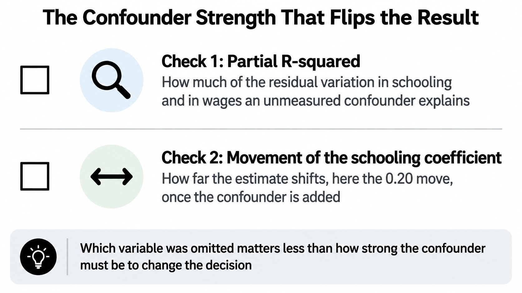
The two checks below answer different questions and should never be collapsed into one sentence.
Two checks, reported separately
Partial R² sensitivity analysis, in the sense of Cinelli and Hazlett, asks how much of the residual variation in the outcome and in the treatment an unmeasured confounder would have to explain to move your estimate to zero, or to a threshold you choose. It's a statement about omitted explanatory power, in units a reader can argue with.
An Oster-style coefficient-stability bound works differently. It compares a short and a long regression and scales the movement in the coefficient by how much R² improved, relative to a benchmark R² the researcher states up front. The output is a claim about how much selection on unobservables would have to matter relative to selection on observables.
Both are useful. Merging them is not, because they can disagree, and a reader can't tell which one you meant.
Set the threshold before the estimate
Return to the wage sketch. Suppose the decision hinges on a schooling return of at least 0.05, and your best controlled estimate is about 0.08. The number worth reporting isn't only the confounder strength that drives the estimate to zero, since zero isn't the decision boundary. It's the strength that drives 0.08 down to 0.05.
That distinction changes conclusions. A confounder strong enough to erase the effect entirely may be implausible. One strong enough to erase the margin over the threshold may be entirely plausible. Reporting only the first flatters the finding.
The tipping point belongs in the same sentence as the coefficient, not in an appendix paragraph about limitations. Routine implementations exist, sensemakr among them, and a hand calculation off the partial R² is enough for a first pass.
Tipping-point reporting: "an unmeasured confounder would need to explain X% of the residual variation in both schooling and wages to move this estimate below 0.05." If you can't fill in X, the analysis isn't finished.
When the answer is different data
Recent work on omitted-variable and sensitivity practice frames the applied decision around two questions: which variables should have been measured, and which plausible confounders remain once measurement constraints are acknowledged. That reframing is deliberately contrarian. When a weak unmeasured confounder could overturn the estimate, the right response may be to collect different data or narrow the research question rather than adding covariates to the same observational model.
The same paper pushes against treating omitted-variable bias and measurement error as separate textbook chapters. When the stand-in variable is noisy, the two problems arrive together, and a sensitivity analysis that assumes a clean omitted confounder misses half the exposure.
None of this identifies anything. Sensitivity analysis doesn't replace a design, and a good design doesn't excuse an unreported tipping point. Directed acyclic graphs, negative controls, fixed effects, and instruments all stay in the toolkit. What changes is that the number travels with the coefficient. Worked versions of this reporting style are collected in these sensitivity analysis examples.
Write the Identification Memo Before You Cite the Estimate
A memo is six lines, written before anyone cites the coefficient.
- The suspected omitted factor and the open back-door path. Name the variable and the two arrows.
- The predicted sign of βz × δ. Taken from the sign table, recorded before the long model was fit.
- The short and long estimates. Roughly 0.28 and 0.08 in the simulated wage case, with the 0.20 gap accounted for rather than noted.
- The remedy used. A measured control, a fixed effect, an instrument, or a decision to collect new data.
- The confounder strength that crosses the decision threshold. State whether the figure is a partial R² result or an Oster bound, because they aren't interchangeable.
- Whether the stand-in is a noisy proxy. If it is, record that measurement error can flip the direction of whatever bias remains. An imperfect proxy is not automatically safer than leaving the column out.
Each line forecloses a specific objection. The sign line blocks "you never checked direction." The proxy line blocks "you added a control and called it identified." Once the six lines exist, the sensitivity table reports a tipping point instead of a gesture, and the figure caption can carry the confounder strength that would move the estimate past the threshold.
If you want help executing a specification you've already chosen, PlotStudio AI runs it through agentic analytics: agents plan the investigation, execute Python locally, inspect intermediate regressions, revise the approach when something fails, and save a reproducible Analysis Page with code, charts, and statistics. Verification Mode lets you review the plan before anything runs, propose your own methodology, edit it directly, see a diff summary of every change, and undo any edit in one click. Domain methods are applied automatically, including IV/2SLS for causal inference. The Effortless Academic review is a product walkthrough rather than a methods reference.
Try PlotStudio AI when you're ready to run a specification you've already defended.