Most guides treat the treatment effect on the treated as a minor variant of ATE. That advice is too loose for applied work. If your policy reached a specific subgroup, ATT is usually the estimand that matches the question, and the rest of the analysis lives or dies on whether you can identify it cleanly, estimate it without hidden balance problems, and report it in a way reviewers trust.
Why the Treatment Effect on the Treated Deserves Its Own Number
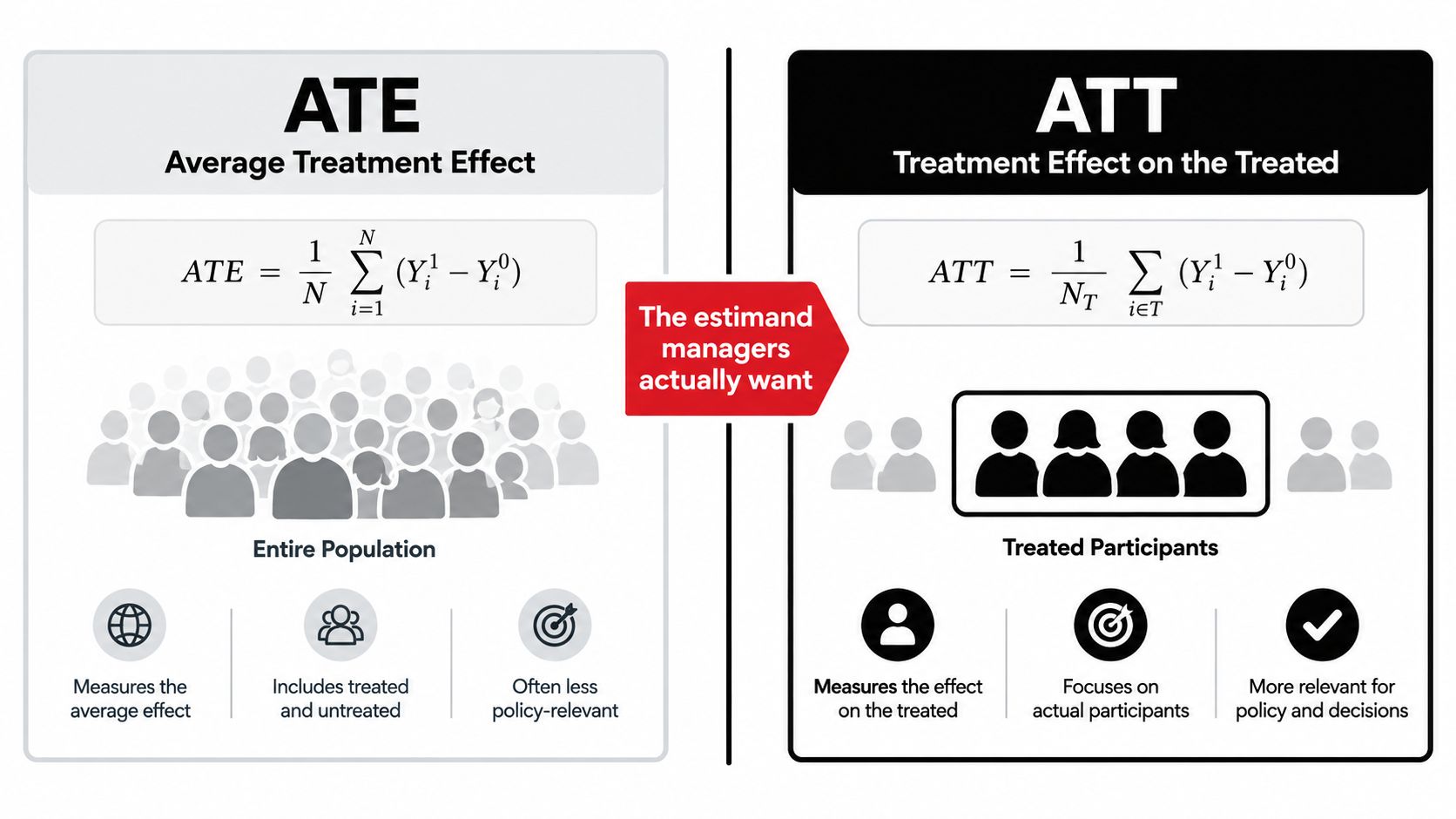
The most common mistake is to act as if ATE and ATT are interchangeable. They are not. ATE asks what would happen if everyone were treated, while ATT asks what happened to the people who received the treatment. In evaluation work, that distinction matters because program managers rarely care about a hypothetical full-population rollout before they know whether the first cohort benefited.
A job-placement rollout in one district makes the difference concrete. If only district 1 received the program, the manager wants the effect on those participants, not a population-average number that mixes treated workers with people who never had access. That is why ATT often carries the right policy interpretation, especially when treatment selection is non-random and the treated subgroup is not representative of the broader sample.
The three estimands people mix up
The full discussion usually involves ATE, ATT, and LATE. ATE is the average effect over the whole population, ATT is the average effect among treated units, and LATE is the effect for compliers under a variable-based approach. Those three are not cosmetic variants, they answer different policy questions and can diverge when treatment effects are heterogeneous.
Practical rule: if your paper's question begins with “among the units that actually got treated,” ATT is the first estimand to check, not an afterthought.
A single regression coefficient rarely settles the issue. If treatment effects vary across units, the coefficient from a standard model is usually some weighted average with its own interpretation, not automatically the estimand your reader thinks you reported. That is why the estimand should come first, before the estimator, before the standard errors, and before the plots.
Formal Definitions of ATT, ATE, and LATE in One Notation
The potential-outcomes setup
Write the potential outcomes as Y(1) for the outcome under treatment and Y(0) for the outcome under no treatment. Let D = 1 indicate treatment and D = 0 indicate control. The observed outcome is one realized value from that pair, but the unobserved counterfactual remains missing for each unit.
The estimands then follow directly. ATT = E[Y(1) − Y(0) | D = 1], ATE = E[Y(1) − Y(0)], and LATE = E[Y(1) − Y(0) | complier]. The point of writing them this way is that the conditioning set changes the target population, which changes the substantive claim you can make.
| Estimand | Conditional population | Policy question | Equality condition |
|---|---|---|---|
| ATT | Treated units | What did treatment do to those who got it? | Equals ATE only when effects are constant across treatment status |
| ATE | Entire population | What if everyone were treated? | Equals ATT only under effect homogeneity |
| LATE | Compliers | What did the instrument do for units moved by assignment? | Equals ATT only in special designs, not generally |
Why ATT and ATE separate in practice
ATT and ATE coincide only in the special case where treatment effects do not vary across the relevant subgroups. Once effect heterogeneity enters, the treated group can have a different average gain than the whole population, even if the treatment itself is unchanged. That is the central reason to stop using “the treatment effect” as if it had one universal meaning.
For a policy question, the target is the object that answers the policy question. If the question is about an existing program's participants, ATT is the right estimand. If the question is about a universal rollout, ATE is the right one. If assignment is instrument-driven and the question is about compliers, LATE is the correct target.
The notation matters because it stops researchers from changing the estimand after the fact. I'd rather see a paper choose the right target and defend it than see one estimate reported as if it answered every causal question at once. For a broader causal workflow, see the causal inference guide.
Identification Assumptions That Make ATT Estimable
The three assumptions in plain language
ATT is estimable only if you can reconstruct the missing counterfactual for the treated group from comparable untreated units. In observational data, that typically requires three assumptions. First, untreated outcomes for treated and untreated units must be comparable after conditioning on observed covariates. Second, every relevant covariate profile must contain both treated and untreated units often enough to support the comparison. Third, one unit's treatment must not change another unit's outcome.
In symbols, the first assumption is unconfoundedness, written as Y(1), Y(0) ⊥ D | X. The second is overlap, written as 0 < P(D = 1 | X) < 1. The third is SUTVA, the Stable Unit Treatment Value Assumption, which rules out interference and hidden versions of treatment. The logic is simple, but the cost is high, because unconfoundedness rules out unobserved confounding.
Key implication: if treated units self-select because of motivation, severity, or need, then ATT becomes an identification problem, not just an estimation problem.
Where each assumption breaks
Self-selection into job training is the classic failure mode. The treated group often differs from the untreated group on unmeasured factors that also affect outcomes, and no amount of regression adjustment fixes bias from variables you never measured. Overlap fails when some covariate profiles are almost always treated or almost never treated, which makes comparison unstable for ATT because the estimand focuses on the treated subgroup only.
SUTVA is the assumption researchers forget first. It breaks in settings with spillovers, network effects, geographic contamination, or crowding out. If a treated school changes neighboring schools' outcomes, then the untreated counterfactual is no longer clean, and the ATT target itself becomes ambiguous.
For a method that often sits in the background of these discussions, the instrumental variable regression guide is a useful companion. It helps separate identification through instruments from identification through selection-on-observables, which are not the same problem.
Choosing an Estimator for ATT in Observational Data
Match the estimator to the data structure
No single estimator dominates across settings. When covariates are few and overlap is good, matching can be transparent. When the outcome model is credible and the functional form is defensible, regression adjustment can be efficient. When the treated group is the target population and direct weighting is the goal, inverse probability weighting is a natural choice. In harder observational settings, doubly reliable estimators such as AIPW or TMLE often deserve serious consideration because they can still perform well if one nuisance model is misspecified.
Each option has a failure mode, and reviewers usually want to see that you know it. Matching is intuitive, but it can deteriorate quickly as the covariate space widens, because nearest neighbors stop being close. Propensity-score matching reduces the dimension of the problem, yet it still depends on a believable score model and enough overlap. Regression adjustment is easy to explain, but it can mislead if the outcome model is misspecified. IPW is elegant in form, though it becomes unstable when estimated treatment probabilities are near zero or one.
| Estimator | Identification | Behavior When a Model Is Misspecified | Software |
|---|---|---|---|
| Matching | Selection on observables plus overlap | Moderate, sensitive to poor matches | Common in R and Python |
| Regression adjustment | Correct functional form for outcome model | Lower if the model is wrong | Very broad |
| IPW | Correct propensity model plus overlap | Sensitive to extreme weights | Broad |
| AIPW or TMLE (doubly robust) | Either outcome or propensity model can be right | Better than single-model approaches | Broad |
| IV or LATE methods | Valid instrument and monotonicity-style logic | Different estimand, not ATT | Broad |
Why AIPW and TMLE often become the default
For ATT work in observational data, doubly safeguarded estimators are attractive because one bad nuisance model does not automatically invalidate the analysis. That does not remove the need to diagnose balance or inspect model fit. It just lowers the risk that a single modeling error will drive the result.
The appeal grows when D is large relative to N, or when treatment selection is clearly non-random. In those settings, the analyst often needs flexible nuisance models while still preserving the estimand. AIPW and TMLE are often the default because they give that combination more cleanly than a single-model approach.
PlotStudio AI can fit into that workflow when you want a tool that plans and runs a multi-step ATT analysis, executes Python locally, and saves the result as a reproducible analysis page. That kind of agentic analytics is useful when the analysis needs balance checks, model revisions, and documentation rather than a single shortcut answer.
Estimating ATT with Difference in Differences
The 2 by 2 logic
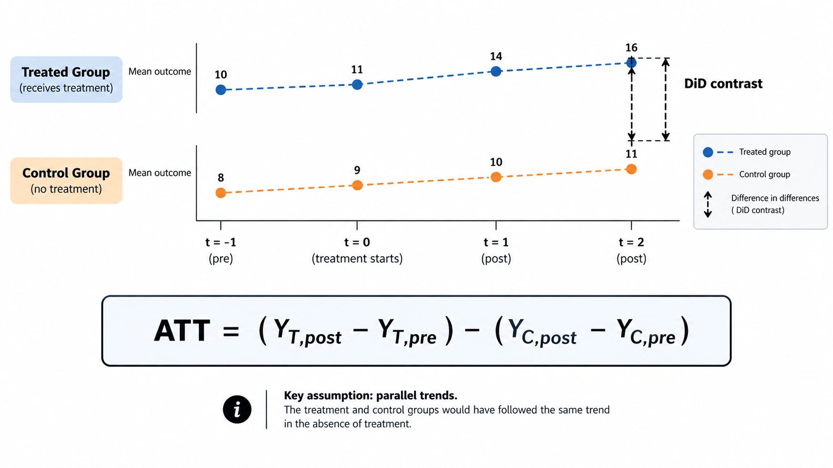
Difference in differences works when treated and control groups would have followed parallel trends absent treatment. In the simplest two-group, two-period setup, the ATT is the post-pre change for the treated group minus the post-pre change for the control group. The time effect gets differenced out, leaving the treatment effect under the identifying assumption that the untreated trend is shared.
That assumption is about trends, not levels. Treated and control units can start at very different outcome levels and still satisfy parallel trends if the gap would have stayed stable in the absence of treatment. Researchers often get this backwards and over-focus on baseline differences that do not matter for the identification argument.
Event studies and staggered adoption
In staggered adoption settings, the event-study form is often more informative than a single static coefficient. A common specification is Y_it = α_i + γ_t + Σ_k β_k 1[t − T_i = k] + ε_it, where the coefficients trace dynamic effects relative to treatment timing. In modern practice, cohort-specific ATT(g,t) is usually the right interpretive object, because treatment timing varies and a pooled coefficient can hide substantial heterogeneity.
The diagnostic everyone should inspect is the pre-period pattern. If the lead coefficients are drifting before treatment, parallel trends looks shaky. Heterogeneous timing also creates weighting problems in two-way fixed effects, so methods associated with Goodman-Bacon decomposition, Callaway-Sant'Anna, and Sun-Abraham exist to recover cleaner cohort-time effects.
Here's the video version of the same logic if you want a visual reminder of the 2x2 contrast.
For panel workflows, the panel data analysis guide is the natural companion. Use cluster-level standard errors at the unit level when units are followed over time, and be explicit about whether your control group is never-treated or not-yet-treated, because that choice changes the comparison set.
Diagnostics, Robustness Checks, and Reproducible Code
Balance and placebo checks you can defend
If you estimate ATT with matching or weighting, start with covariate balance. Standardized mean differences and variance ratios tell you whether treated and weighted controls are close enough on observed covariates to support the design. A common practical threshold is an SMD below 0.1, and a love plot makes the before-after pattern easy to inspect without forcing the reader to parse a wall of coefficients.
Balance diagnostics are not decorative. They are your first test of whether the comparison group actually looks like a counterfactual.
Placebo tests belong right next to balance checks. Use pre-period outcomes, pseudo-treatment dates, or permuted treatment assignment to see whether your design generates effects when it should not. If a placebo analysis lights up, your main ATT estimate needs a harder look before anyone writes the abstract.
Sensitivity analysis and reproducible pipelines
Unobserved confounding never disappears just because the main estimate is statistically neat. Rosenbaum bounds help you ask how strong hidden bias would need to be to overturn the result, and an omitted-variable bias sensitivity analysis such as the Cinelli-Hazlett style slope analysis gives another way to communicate fragility. Report those results when the design depends heavily on selection-on-observables.
A reproducible workflow should store the fitted propensity model, the random seed, and package versions, then reuse them for balance tables, AIPW estimation, and placebo DiD runs. In Python, that can involve scikit-learn, econml, causaldata, and plotnine. In R, the usual stack includes MatchIt, WeightIt, did, and fixest. The point is not the package list, it's that the estimation, diagnostics, and figures come from one auditable pipeline.
For reproducibility norms in research workflows, the research reproducibility guide is the right reference point. If your analysis is going to survive review, every check should map to a specific failure mode, and every output should be re-runnable from code alone.
Common Pitfalls When Reporting ATT in Papers
The mistakes reviewers spot fast
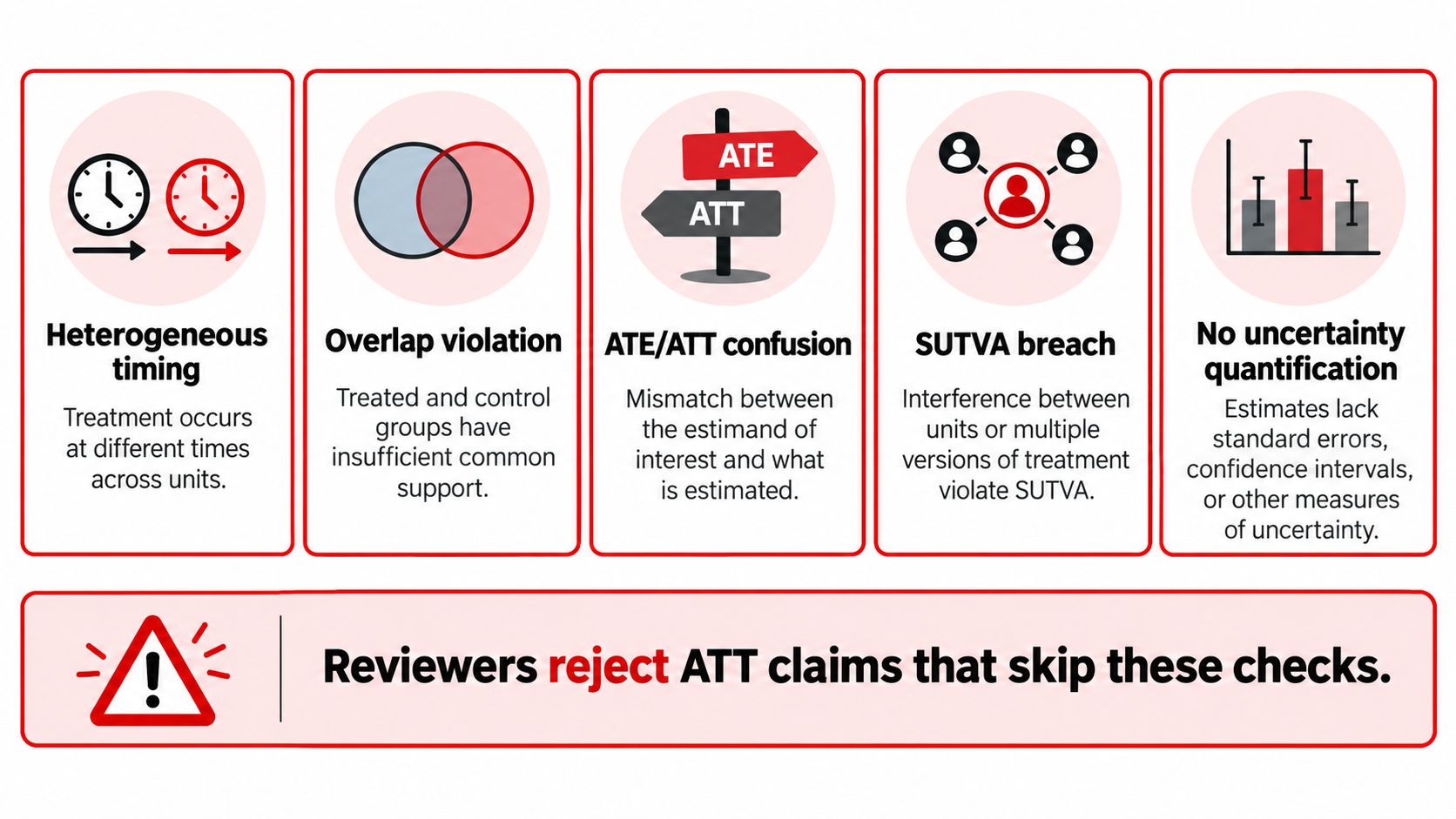
The first error is confusing ATT with the output of a two-way fixed-effects regression when treatment timing is staggered. That model can mix already-treated and not-yet-treated units in ways that distort the weighted average. The fix is to report cohort-time effects or a modern staggered-adoption estimator instead of a single summary coefficient.
The second is ignoring overlap problems. If weights explode, the ATT estimate can become numerically unstable and substantively unconvincing. The diagnostic is the weight distribution, and the fix is trimming, restricting support, or revisiting the estimand if the target population is too sparse.
| Pitfall | Diagnostic | Minimal fix |
|---|---|---|
| Heterogeneous timing | Event-study coefficients, cohort-time plots | Use modern staggered-adoption estimators |
| Overlap violation | Extreme weights, sparse covariate cells | Trim or redefine support |
| ATE and ATT confusion | Target-population statement missing | State the estimand explicitly |
| SUTVA breach | Spillover evidence, geographic contamination | Redesign comparison groups |
| No uncertainty quantification | Missing SEs or intervals | Report robust uncertainty measures |
Estimand discipline matters
A third problem is reporting a point estimate without defining the target population. If the reader cannot tell whether the number is ATT, ATE, or LATE, the result is hard to interpret and easy to misread. Another common failure is to present an ATT claim from an IV design as if it were a direct treated-group average, which it is not.
If the paper uses DiD, omitting pre-trend evidence is an avoidable mistake. If it uses IV, weak instruments need to be shown, not implied. Reviewers don't need perfection, but they do need to see that you know which threats your design can address and which ones it can only bound or probe with sensitivity checks.
Putting ATT to Work in Your Research Workflow
A paper-ready sequence
A clean ATT workflow has five deliverables. First, define the estimand in writing before estimation starts. Second, justify the estimator with respect to the data structure and the identification assumptions. Third, report diagnostics such as balance tables or pre-trend plots. Fourth, include an appendix with alternative specifications and sensitivity checks. Fifth, use reporting language that names the target population and the assumptions behind it.
That sequence is more than bureaucracy. It forces the analysis to match the question, and it helps reviewers see that the claim is narrower, and stronger, than a generic treatment-effect statement. For empirical research, that discipline usually matters more than whichever single estimator you chose first.
Where agentic analytics helps
This is also the kind of workflow where agentic analytics earns its keep. A system like PlotStudio AI can plan the estimation path, run the code locally, inspect intermediate output, revise the analysis if balance fails, and save the final results as a reproducible Analysis Page. That doesn't replace judgment, but it does reduce the chance that balance checks, plots, and code drift apart across drafts.
The best reporting standard is the one another researcher can rerun without asking you for hidden steps.
If you want a one-page checklist, use this order: define ATT, verify identification, select the estimator, run diagnostics, test sensitivity, and write the results in terms of the treated population. Then archive the code, the settings, and the outputs together so the analysis can be audited later.
If you're building an ATT analysis for a paper, thesis, or policy memo, start with the estimand, not the estimator. Then run the diagnostics that match your design, document the assumptions you're relying on, and keep the workflow reproducible from the first model to the last figure. If you want software that can help execute and document that pipeline, try PlotStudio AI at plotstudio.ai with 1,000 free credits for researchers and researcher pricing at the academic plan.