You're looking at support tickets, hospital visits, defects, or claims, and the outcome is a nonnegative count. Poisson regression models are designed for that setting: they model an expected count with a log link, making predictor effects multiplicative rather than additive. They're a strong starting point when events are countable and exposure is measured correctly, but diagnostics determine whether Poisson is sufficient.
PlotStudio brings this work into agentic analytics, where an AI data analyst plans a multi-step investigation, writes and runs real Python locally, checks the output, and saves a reproducible Analysis Page. An answer is a data point. An analysis is actionable, auditable intelligence that includes the reasoning path, charts, code, and statistical checks.
Table of Contents
- Introduction to Poisson Regression Models
- What Poisson Regression Models Are and How They Work
- Core Assumptions and When They Break
- Estimation Interpretation and Inference in Practice
- Diagnostics Goodness of Fit and Overdispersion Checks
- Choosing Extensions for Overdispersion and Excess Zeros
- Applied Examples Reproducible Code and Common Pitfalls
Introduction to Poisson Regression Models
A common situation is deceptively simple. You have the number of customer contacts per account, readmissions per patient, or manufacturing defects per batch, and you want to understand which predictors are associated with higher or lower counts. Ordinary linear regression may produce negative fitted values, treats changes as additive across the entire outcome range, and imposes a variance structure that often doesn't fit event data.
Poisson regression addresses the first two problems through a generalized linear model. It models the conditional mean count, keeps predictions nonnegative through an exponential link, and expresses effects on a rate or expected-count scale. That makes it useful for incidents, claims, complaints, visits, failures, and other outcomes where zero and positive integers have direct meaning.
The important qualification is that Poisson regression isn't automatically the final model. Its classical variance assumption is restrictive, and real data often contain clustering, unobserved heterogeneity, bursty events, or more zeros than a basic Poisson distribution can explain. A responsible workflow therefore starts with Poisson, checks dispersion and residual behavior, and then considers quasi-Poisson, negative binomial, zero-inflated, or hurdle alternatives.
This guide develops that workflow from the ground up. You'll see how the distribution and log link work, how to use offsets when exposure differs, how to interpret coefficients as incidence-rate ratios, and how to separate overdispersion from structural zeros. The aim isn't to memorize a formula. It's to know what question each model answers and what evidence justifies moving beyond the default.
For researchers, analysts, and consultants, reproducibility matters as much as estimation. PlotStudio is built like a researcher rather than a chatbot. You can upload a dataset, review the proposed methodology in Plan Mode, inspect the generated Python, and return to a saved Analysis Page instead of losing the result inside a chat thread. Its local Python engine keeps data on your machine, while the saved page preserves narrative, charts, code, and statistics for later review or export.
What Poisson Regression Models Are and How They Work
Start with the outcome. A Poisson response represents the number of events occurring in a defined observational window, such as tickets per account-month or defects per production batch. The model assumes that, conditional on the predictors, the response follows a Poisson distribution with an expected value that depends on those predictors.
The generalized linear model formulation is:
[
\mu_i = \exp(x_i\beta)
]
Here, (\mu_i) is the expected count for observation (i), (x_i) is its predictor vector, and (\beta) contains the coefficients. Taking logarithms gives the linear predictor:
[
\log(\mu_i)=x_i\beta
]
This is the log link. The predictors combine linearly on the log-mean scale, but their effects become multiplicative after transforming back to the count scale. A coefficient of (\beta_j) changes the expected count by the factor (\exp(\beta_j)) for a one-unit increase in predictor (x_j), holding other variables constant.
Why the log link fits event rates
Think about event intensity rather than raw totals. If one account has twice the opportunity to generate tickets because it was observed for twice as long, its expected ticket count should scale with exposure. Likewise, a predictor that increases an incident rate should have a proportional effect across the relevant range, not a fixed number of added events for every observation.
This is why Poisson models are often used for incident counts, defect counts, claim counts, and event frequencies. The log link guarantees a positive expected mean and naturally represents compounding effects. A predictor effect that is constant on the log scale becomes a rate multiplier on the original scale.
The framework sits within generalized linear modeling. Poisson regression became a formal statistical workhorse in the 1970s, after John Nelder and Robert Wedderburn unified generalized linear models in 1972, providing the modern likelihood-based framework for count outcomes and log-link mean structures. The model's likelihood also supports deviance-based fit assessment and related pseudo-(R^2) measures, as described in this overview of Poisson regression.
Core idea: Poisson regression is linear in predictors on the log-mean scale, not on the raw count scale.
Offsets convert counts into rates
Raw counts aren't comparable when observations have different exposure. If one hospital ward is observed for a longer period, or one policy covers more exposure time, the model needs that known scaling information.
An offset adds the logarithm of exposure with its coefficient fixed at one:
[
\log(\mu_i)=\log(\text{exposure}_i)+x_i\beta
]
In software, that often appears as offset(log(exposure)). The offset isn't an ordinary predictor whose effect is estimated. It tells the model that expected events should be proportional to known exposure, allowing the remaining coefficients to describe differences in event rates. This multiple regression primer provides useful background on how this count-model formulation extends the broader regression framework.
Under the classical Poisson assumption, the variance equals the mean:
[
\operatorname{Var}(Y_i)=\operatorname{E}(Y_i)=\mu_i
]
That relationship is convenient when it reflects the data. It's also the assumption most likely to require scrutiny.
Core Assumptions and When They Break
A hospital records many patient contacts, a support team counts customer requests, and a factory logs defects. In each case, Poisson regression asks how predictors change the expected count after accounting for exposure. Its assumptions matter because a plausible average can still produce misleading uncertainty or hide a missing data-generating process.
Equidispersion is the first checkpoint
The classical model assumes:
[
\operatorname{Var}(Y_i)=\operatorname{E}(Y_i)
]
This property is equidispersion. When observed variation exceeds the fitted mean, the counts are overdispersed. Ordinary Poisson standard errors may then be too small, producing confidence intervals that are too narrow and significance tests that appear stronger than the evidence supports.
The extra variation often has a substantive cause. Patients treated in the same hospital may share unmeasured conditions, some customers may be unusually likely to contact support, or one event may trigger several later events. Omitted interactions and unmodeled heterogeneity create the same pattern. Underdispersion can occur in tightly controlled processes, where counts vary less than the Poisson model permits.
A quasi-likelihood approach can adjust for dispersion while retaining the mean structure. A negative binomial model is better suited when the excess variation reflects a different count distribution rather than only a scale problem.
Independence and the unit of analysis
Observations should be independent after conditioning on the modeled predictors, or the analysis should represent their dependence directly. Repeated records from one customer, measurements from one patient, and defects from one production line can share latent causes.
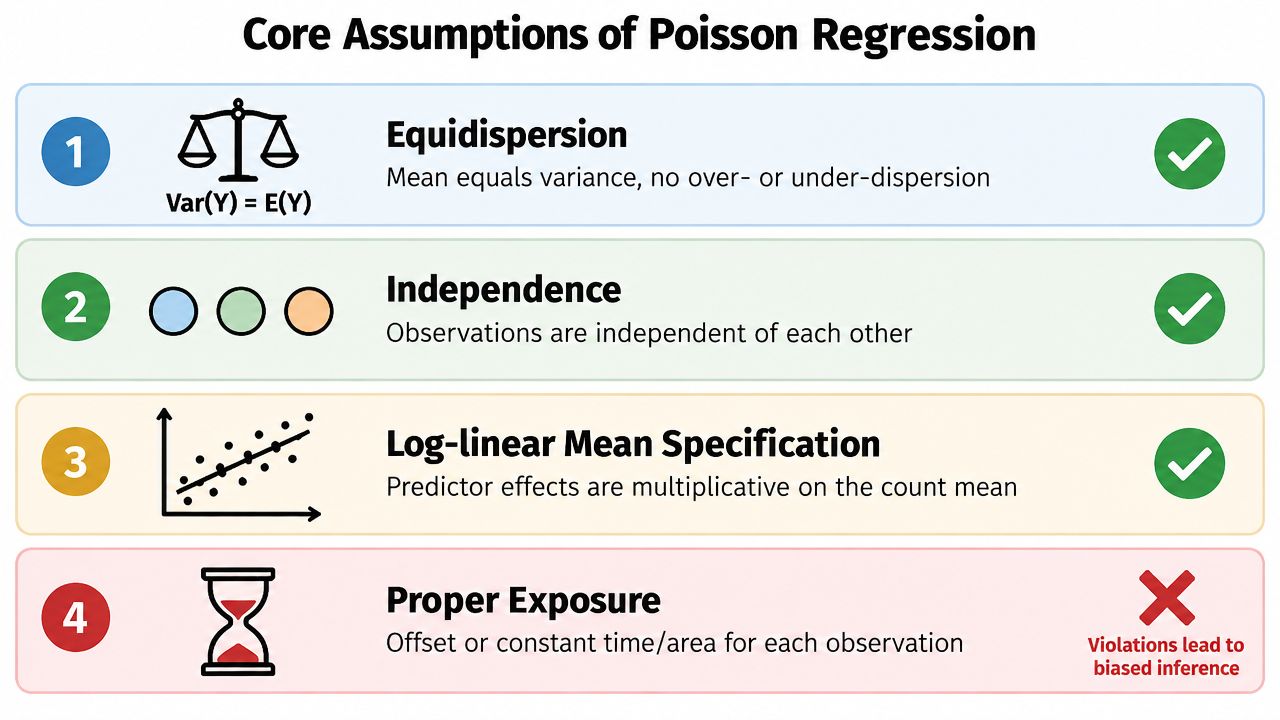
A clustered dataset may require cluster-adjusted covariance, random effects, or a model for the grouping process. Adding rows does not create more independent evidence. If dependence is ignored, coefficient estimates can look reasonable while their uncertainty is understated.
The mean specification must be credible
The log-linear specification requires predictors to combine linearly on the log scale of the expected count. A nonlinear effect, omitted interaction, or unsuitable functional form can leave a recognizable pattern in the residuals.
Examine residuals against fitted values and important continuous predictors. Curvature suggests a missing nonlinear term. A fan-shaped pattern suggests changing variability, while groups with consistently positive or negative residuals suggest omitted structure. Transformations, splines, interactions, or domain-specific variables may improve the conditional mean before you change the response distribution.
Exposure must be represented correctly
If follow-up time, population at risk, operating hours, or another known exposure differs across observations, include an offset. Otherwise, a longer observation window may be mistaken for a higher underlying event rate.
Use the following decision sequence:
- Keep Poisson with corrected standard errors when the conditional mean appears well specified but the variance assumption is doubtful.
- Use quasi-Poisson when the same mean structure is appropriate, a dispersion adjustment is sufficient, and a full likelihood is unnecessary.
- Use negative binomial when excess variance appears to belong to a different count distribution that should be modeled directly.
- Investigate zero-inflated or hurdle models when zeros may arise from a separate structural process rather than ordinary sampling variation.
Compare these choices with reproducible residual checks, dispersion diagnostics, and sensitivity analyses. Poisson is a starting model, not a verdict.
Estimation Interpretation and Inference in Practice
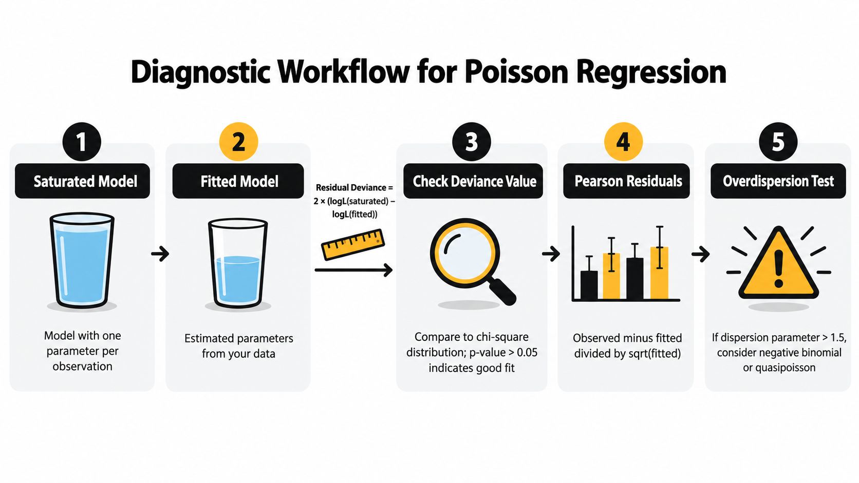
Poisson regression is generally estimated by maximum likelihood. The fitting procedure selects coefficients that make the observed counts most plausible under the specified Poisson likelihood, given the predictors and any offset. The log-likelihood is central to this process, while deviance measures how the fitted model compares with a saturated model that fits each observation as closely as possible.
A coefficient is easiest to interpret after exponentiation. If the fitted coefficient for a binary predictor is (\beta_j), then:
[
\operatorname{IRR}=\exp(\beta_j)
]
This is the incidence-rate ratio. An IRR above one indicates a higher expected rate for the comparison group, while an IRR below one indicates a lower expected rate, conditional on the rest of the model. For a continuous predictor, the IRR describes the multiplicative change associated with a one-unit increase, so the unit itself must be scientifically meaningful.

Report ratios and predicted counts
An IRR is compact, but it isn't always intuitive to a nontechnical audience. A strong report gives both the ratio and predicted means at representative covariate values.
For example, “the expected contact rate is multiplied by (\exp(\beta)) for each additional unit of account complexity” communicates the model structure. Predicted counts for low, typical, and high values of complexity show what that multiplier means in the actual outcome scale. Avoid describing a log-link coefficient as an additive change in tickets, visits, or defects.
The same principle applies to uncertainty. Report coefficient intervals on the exponentiated scale when presenting IRRs, and show predicted-mean intervals when the practical question concerns expected counts. This guide to interpreting regression results covers the broader discipline of separating statistical scale from practical interpretation.
The offset deserves special care:
count ~ predictors + offset(log(exposure))
The offset's coefficient is fixed at one. Treating log(exposure) as an ordinary covariate estimates an exposure effect instead of enforcing the known proportional scaling required for a rate model.
Inference when variance is misspecified
Wald tests use coefficient estimates and their standard errors. Likelihood-ratio tests compare maximized likelihoods between nested models. Both can be useful, but their reliability depends on the variance and likelihood assumptions that support them.
When the mean model is credible but equidispersion fails, a sandwich covariance estimator is a practical correction. The coefficient estimates usually remain similar, while the standard errors become more reliable under variance misspecification. For clustered records, the covariance should also reflect the grouping structure.
A clean result table should identify the response, exposure definition, link, model family, coefficient scale, uncertainty method, and diagnostic evidence. Readers need to know whether an apparently strong association survives a variance correction, not just whether the original Poisson p-value crossed a threshold.
Diagnostics Goodness of Fit and Overdispersion Checks
Treat model checking as a detective process. First inspect the fitted values and residuals, then quantify deviance and dispersion, and finally connect any failure to a modeling decision. A single significant test shouldn't replace substantive diagnosis.
Deviance measures distance from a perfect fit
For Poisson regression, residual deviance is defined as:
[
D=2{\log L_{\text{saturated}}-\log L_{\text{fitted}}}
]
The saturated model gives each observation the flexibility needed for a perfect fit. The fitted model uses the restrictions imposed by the predictors. Residual deviance therefore summarizes how much likelihood is lost by using the model rather than the saturated benchmark.
Inspect deviance alongside residual degrees of freedom, but don't treat a single comparison as decisive. Large values can reflect omitted structure, exposure problems, influential observations, or a variance distribution that is too narrow.
Calculate a dispersion estimate
A common diagnostic divides Pearson chi-square or residual deviance by residual degrees of freedom. Values much larger than one indicate overdispersion and suggest that conventional Poisson inference may be unreliable.
The visual checks add context:
- Residuals versus fitted values: Look for widening spread or systematic curves.
- Residuals versus predictors: Search for nonlinearity and omitted interactions.
- Observed versus predicted counts: Identify whether the model misses high-count observations or produces too few zeros.
- Grouped summaries: Compare mean and variance across meaningful strata, especially exposure bands.
A dispersion correction can be written as:
[
\operatorname{Var}(Y_i)=\sigma^2\mu_i
]
with (\sigma^2>0). Under a quasi-Poisson-style adjustment, the coefficient covariance matrix is multiplied by the estimated dispersion, while test statistics and residual scaling are adjusted accordingly. This changes inference without necessarily changing the fitted mean.
The regression diagnostics workflow in PlotStudio can be useful when you want profiling, residual plots, dispersion checks, and narrative interpretation captured in one saved Analysis Page. That differs from a one-shot chat answer, which may return a formula without preserving the checks needed to defend the result.
Choosing Extensions for Overdispersion and Excess Zeros
Model selection should begin with the failure mechanism. A support-ticket dataset may show counts that vary more widely than their fitted means, while a clinical dataset may contain many zeros because some subjects could never experience the event. These patterns can look similar in a residual plot, yet they call for different models. Dependence among observations adds another possibility.
| Diagnostic signal | Model choice | Why it fits |
|---|---|---|
| Mean structure is credible, variance is misspecified | Poisson with corrected SEs | Keeps the Poisson mean model while correcting covariance estimates |
| Dispersion differs from the strict Poisson assumption | Quasi-Poisson | Adds a dispersion parameter for inference without changing the mean structure |
| Variance exceeds the mean and a full likelihood is useful | Negative binomial | Adds a variance structure designed for overdispersed counts |
| Excess zeros arise from a distinct “never-event” process | Zero-inflated model | Separates structural zeros from the ordinary count process |
| Zeros and positive counts follow separate mechanisms | Hurdle model | Models reaching a positive count separately from the size of that count |
| Binary outcome, risk-ratio target, clustered setting | Modified Poisson with caution | Estimates association or causal risk ratios, subject to probability calibration checks |
Poisson with corrected SEs and quasi-Poisson choices
A Poisson model with corrected standard errors is appropriate when the expected-count relationship and exposure offset remain defensible, but the variance assumption is too narrow. The fitted mean stays the same. Only the uncertainty calculation changes, much like keeping a route while correcting the estimated travel time.
Quasi-Poisson goes one step further by estimating a dispersion multiplier for the variance. It retains the Poisson-style mean structure, but it does not define a complete likelihood in the usual way. AIC and BIC may therefore be unavailable or inappropriate for comparing these semiparametric alternatives. Choose it when inference about the mean relationship matters more than full probabilistic prediction.
Negative binomial and zero processes
Negative binomial regression is a candidate when unobserved heterogeneity or other count-level variation makes the variance exceed the mean. A comparative count-model study reports improved fit over Poisson in overdispersed settings and discusses zero-inflated negative binomial models when excess zeros occur alongside overdispersion.
A zero-inflated model represents two generating processes: one produces structural zeros, and the other produces ordinary counts, including possible sampling zeros. A hurdle model also separates zero from positive outcomes, but treats the positive counts as a distinct conditional process. The choice should follow the event story. If some accounts can never generate a ticket, structural zeros have a defensible interpretation. If every account could generate one but some did not during observation, a hurdle or ordinary count model may be more suitable.
Modified Poisson regression addresses a different problem. Analysts often use it for binary outcomes when the target is a risk ratio, but predicted probabilities can exceed one. It is therefore better suited to association or causal estimation than to calibrated prediction in some settings. A 2025 study notes that semiparametric Poisson-based methods may not support likelihood-ratio, AIC, or BIC selection in the usual manner, as described in this cluster-weighted modified Poisson preprint.
For a broader treatment of methods and model checks, see advanced statistical methods for applied analysis. Pair the selected model with reproducible comparisons of dispersion, zero frequencies, fitted counts, and prediction behavior.
Applied Examples Reproducible Code and Common Pitfalls
Consider a SaaS team modeling support contacts per account-month. The response is a count, the predictors might include account complexity and product usage, and the exposure is the number of account-months observed. Start with a Poisson model, include the exposure offset, and inspect dispersion before interpreting significance.
A reproducible workflow looks like this:
- Upload and profile: Check missing values, types, duplicated records, and the definition of one observation.
- Review the plan: In PlotStudio's Plan Mode, verify the response, predictors, exposure variable, comparison groups, and intended diagnostics before execution.
- Fit locally: Generate and run Python in the embedded local engine.
- Check the model: Review fitted means, residuals, deviance, and a Pearson-based dispersion estimate.
- Refit if needed: Use sandwich estimators for inference or compare a negative binomial model when the variance structure requires it.
- Save the result: Preserve narrative, charts, code, and statistics in an Analysis Page, then export to Jupyter or PDF.
The interpretation should stay on the correct scale. An exponentiated usage coefficient is a multiplicative change in the expected contact rate, not a fixed number of extra contacts for every account. Predicted counts at representative usage levels make the result easier to evaluate.
A second example involves hospital readmissions where patients have different follow-up times. The count is readmissions, and the offset is the logarithm of time at risk. Patients with longer observation contribute more opportunity for events, so comparing raw counts without exposure adjustment would confuse follow-up duration with readmission propensity.
Common pitfalls are mechanical but consequential:
- Forgetting the offset: Counts become incomparable when exposure varies.
- Estimating exposure as a regular predictor: This changes a fixed rate adjustment into an estimated association.
- Reading log-scale coefficients additively: Exponentiate coefficients and report incidence-rate ratios.
- Ignoring overdispersion: Standard errors may be too small even when point estimates look reasonable.
- Treating excess zeros as overdispersion alone: Determine whether a structural-zero or hurdle process is plausible.
- Using Poisson for binary prediction without calibration checks: Modified Poisson can support risk-ratio estimation, but predicted probabilities may exceed one.
- Extrapolating beyond observed predictors: A mathematically valid exponential curve can still be scientifically implausible outside the data range.
For academic and research workflows, reproducibility includes the data definition, exposure construction, model formula, diagnostics, and interpretation. PlotStudio's purpose-built workflow supports local execution and persistent Analysis Pages, so the analysis remains inspectable rather than disappearing after the initial answer. An independent review by The Effortless Academic also describes PlotStudio as a purpose-built tool for research data work, including automatic data-quality evaluation and publication-oriented figures.
If you're working with count outcomes, use PlotStudio AI to upload the dataset, review a Poisson modeling plan, run local Python diagnostics, and preserve the complete analysis for reproducible research. Researchers can also apply for 1,000 free credits for researchers through the dedicated research partners program.