Reading a CSV File in R: Import Steps and Fixes

You've just opened sales_q3.csv in R, the import ran without an error, and the first summary already looks wrong. That is the normal failure mode when reading a CSV file in R. A clean run only proves R parsed the text. It doesn't prove the columns, types, decimals or missing values mean what you think.

Pick the Right R Function for Your File

For most comma separated files with a header row and period decimals, read.csv() or readr::read_csv() will work. Choose base R when you want a data.frame with no extra package, readr when you want a tibble with typed columns and parsing warnings, and data.table::fread() when speed on a very large file matters most.

Reader	Package	Returns	Default separator and decimal	Best fit
read.csv()	base R (utils)	data.frame	comma, period	Standard comma separated file with a header and no extra packages
read_csv()	readr	tibble	comma, period	Typed columns, printed specification and parsing warnings in tidyverse pipelines
read_csv2()	readr	tibble	semicolon, comma	European spreadsheet exports that use comma decimals
read.csv2()	base R (utils)	data.frame	semicolon, comma	Same European layout when readr is not available
fread()	data.table	data.table	detected automatically	Very large files where import speed matters most

What you're actually choosing

read.csv() is a wrapper around read.table() with header = TRUE and sep = ",", so it's the safe default for a standard file. The readr manual describes a dedicated family, read_csv(), read_csv2(), read_tsv() and read_delim(), that parses rectangular files into tibbles and is intended to fail clearly when a file changes unexpectedly.

Practical rule: If the file came from a European spreadsheet, start with read_csv2() or read.csv2() and check the first numeric column before you do anything else.

The running example here is sales_q3.csv, with a header, dates and a few missing values. Each later call reads that same file, so differences come from the reader, not the data. Before analysis, basic data profiling starts with this decision. Leave this step with one function per file variant, chosen before any code runs.

Inspect the File Before You Import It

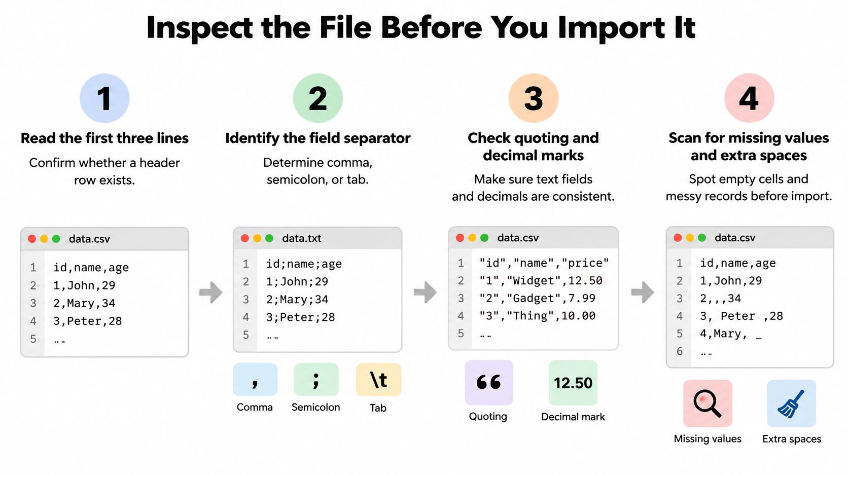
A file named sales_q3.csv can load with no error and still be the wrong table. The first data row becomes the column names, a comma inside a name shifts every later field, or accented text turns into garbage. Excel is the wrong place to look. It rewrites dates, strips leading zeros, and hides quoting, so the evidence you need is gone before you notice.

Open the raw file in a plain text editor and record eight facts. Each one is a choice you will later pass to the reader, and each one needs a check that the file matches what you think you saw.

1. Read the first three lines. Confirm whether a header row exists. If line one looks like data, a default import promotes it to column names and drops a record.
2. Identify the field separator. Comma, semicolon, or tab. The extension will not tell you. A semicolon file read as comma-separated collapses into one wide column.
3. Check the decimal mark. Look for 3.14 versus 3,14. That one character decides between read.csv() and read.csv2().
4. Note problem column names. Spaces, accents, and duplicates get repaired or mangled on import. Write down the originals so you can spot the change.
5. Look for quoted fields. Text that contains commas or line breaks must sit inside double quotes, and every quote must close. An unclosed quote can swallow several rows into one field.
6. Identify the encoding. Search for accented characters and confirm they render correctly. A UTF-8 file may also carry a byte order mark at the very start.
7. Record how missing values appear. Empty fields, NA, N/A, a dot, or a sentinel such as -99 each need different handling later.
8. Count the lines. Run length(readLines("sales_q3.csv")) and compare it with the record count in the source system, allowing for the header and any quoted line breaks.

CSV became a formally documented format in October 2005, when RFC 4180 registered the MIME type text/csv. The RFC describes records on separate lines, fields separated by commas, and optional double quotes, with embedded quotes doubled. It also notes that implementations vary, which is why a clean extension is not a specification.

Say a name field holds Smith, J. Quoted, "Smith, J" is one field. Unquoted, it splits into two and shifts every later column in that row. If you need to inspect or fix the raw text first, an online CSV editor beats a spreadsheet: it shows separators and quotes without rewriting dates. I put the eight findings in the script header. Each one becomes an argument on the import call, so a silent success still has something to check against.

Import Calls for Base R, readr and data.table

Base R first

sales <- read.csv("sales_q3.csv") returns a data.frame. The base R read.table documentation shows read.csv() differs from read.table() mainly through header = TRUE and sep = ",", while read.table() defaults to header = FALSE and whitespace separation. So the call matches read.table("sales_q3.csv", header = TRUE, sep = ",").

That default header is the trap on a headerless file. The first observation becomes the column names, and every later row shifts up by one. Set the names yourself:

sales <- read.csv("sales_q3.csv", header = FALSE,
                  col.names = c("date", "region", "units", "revenue"))

A completed call only means R finished parsing. Check names(sales) against the names you wrote, then nrow(sales) against the export log. If the first data row is sitting in the names, the types below it are already wrong.

readr for typed output

sales <- readr::read_csv("sales_q3.csv") returns a tibble and prints a column specification. That printed spec is why I'd reach for readr on research data. It states, in the console, whether date parsed as a date or stayed character. A value that misses the guessed type raises a parsing warning instead of passing without notice.

Leave the message on for the first import. Read it against the file inspection, then decide whether a finished script may set show_col_types = FALSE. If the spec says double where the source field is an identifier, the read succeeded and the column is still wrong. Fix the type in the call. Do not start summarizing.

data.table when the file is big

sales <- data.table::fread("sales_q3.csv") detects the delimiter and the column types, then returns a data.table. On sales_q3.csv you will not feel the speed. On a large extract you will. Detection is still a guess, and a fast guess can lock in a bad separator or a numeric identifier just as easily as a slow one.

Use fread() when size is the constraint. Keep the same post-import checks you would run on read.csv(). Speed is not a substitute for dim().

Verify all three the same way

Whichever function you chose, stop before any summary:

• Compare dim(sales) with the record count in the source system's export log, or with the file's documented row count.
• Run head(sales) and match the first records to the raw lines you already inspected.
• Run str(sales) and confirm classes for dates, identifiers, and columns that should stay numeric.

If dim() disagrees with that documented count, stop. A read with no error can still drop a quoted row, turn an identifier into a number, or split one field across two columns.

Declare Column Types and Missing Values Up Front

A CSV can finish loading with no error and still be the wrong data. An identifier such as 00123 becomes the number 123, and the leading zeros are gone because R never stored them. A sensor code of -99 enters a model as a real measurement and pulls every mean and coefficient with it. Treat the import as a quality check: declare the type and the missing codes, then prove the file landed that way.

Column content	Base R argument	readr argument
Identifiers	colClasses = "character"	col_character()
Counts	colClasses = 'integer'	col_integer()
Measurements	colClasses = 'numeric'	col_double()
Dates written as dd/mm/yyyy	as.Date(x, format = '%d/%m/%Y') after import	col_date(format = '%d/%m/%Y')
Missing codes such as -99, N/A and a dot	na.strings = c('', 'NA', 'N/A', '-99', '.')	na = c('', 'NA', 'N/A', '-99', '.')

A declaration procedure that holds up

1. Sample first. Read with readr::read_csv("sales_q3.csv", n_max = 1000) and inspect that result with spec().
2. Write col_types explicitly for the production script, column by column.
3. Declare the missing codes with na = c("", "NA", "N/A", "-99", ".") in readr or na.strings in base R.
4. Run problems() on the readr result and compare nrow() with the source record count.
5. For base R, check str() and sapply(df, class) so every class is seen, not assumed.

The readr reference supports explicit settings such as identifiers as col_character(), counts as col_integer(), measurements as col_double() and timestamps as col_datetime(). It also notes automatic guessing examines 1,000 values distributed across the file, so a rare malformed value or a late identifier can still be misclassified. spec() on the sample shows the guess. problems() on the full read shows where a declared type rejected a value.

A guessed type is a hypothesis about your file. A declared type is a test of it, because a value that violates the declaration surfaces in problems().

Base R needs the same check. The R Data Import/Export manual documents na.strings = "NA" as the default, accepting a vector such as c("", "NA", "N/A", "."). Custom tokens in character columns stay ordinary text unless you list them. Leave -99 off that vector and it stays a number.

Run the before-and-after count once. Call sum(is.na(sales$revenue)) and mean(sales$revenue, na.rm = TRUE), reimport with -99 declared missing, and run both again. The NA count rises and the mean moves to the value the remaining observations support. Sound missing data handling starts at import, not at the model.

Keep that full specification in the script so every rerun produces the same column types. A written rule is what makes the result auditable, the same reason a coverage note such as ETF Shariah screening coverage states its decision instead of leaving it implicit.

Fix Encoding, Delimiter and Decimal Problems

The classic silent failure takes ten seconds to detect. Read a semicolon file with read.csv() and you get no error, just one column whose name contains every semicolon from the header line. Check ncol() first, always.

Symptom	Likely cause	Fix
One column holding every semicolon	Semicolon file read with the comma separator	read.csv2() or read_csv2()
Numbers stored as text with comma decimals	European decimal mark read as a period file	locale(decimal_mark = ',') in readr or read.csv2()
Accented names appear as é or similar	File encoding differs from the assumed encoding	fileEncoding = 'UTF-8' or 'latin1', or locale(encoding = 'windows-1252') in readr
Byte order mark sticks to the first column name	UTF-8 file saved with a BOM	fileEncoding = 'UTF-8-BOM'
First data row used as column names	File has no header row	header = FALSE with col.names
Rows with too many or too few fields	Unquoted commas or inconsistent quoting	Inspect with readLines(), correct the source, then check with fill = FALSE

Encoding is the one you can't guess

CSV files carry no reliable metadata about their character encoding. The R Data Import/Export manual warns that automatic detection of many 8-bit encodings is not certain, and that BOMs can cause problems in Unicode files. Base R also documents read.csv2() and read.delim2() for locales where commas are decimal marks and semicolons separate fields.

So trial and error with encodings isn't a fix, it's a lottery. Ask whoever produced the file, or test against a known accented value and record the winning encoding in the script header. Excel exports, institutional systems and legacy software all make different choices, so a collaborator's file needs its own check even when yours imports cleanly. This is core data cleaning work, not cosmetic tidying.

For malformed rows, pull the offending lines out with readLines(), correct the source file or get a clean re-export, and only then test with fill = FALSE so short rows fail loudly instead of being padded. Close with an accent test. Keep one accented name and one decimal value from the raw file in a small check script, and assert both after every import. If either assertion fails, the import is wrong no matter how clean the console looks.

Import Large CSV Files Without Slowing Down

A file of several hundred megabytes can take minutes to load and still hand you the wrong row count. Slow and wrong is the worst combination, and it's common when people optimize the read and skip the checks.

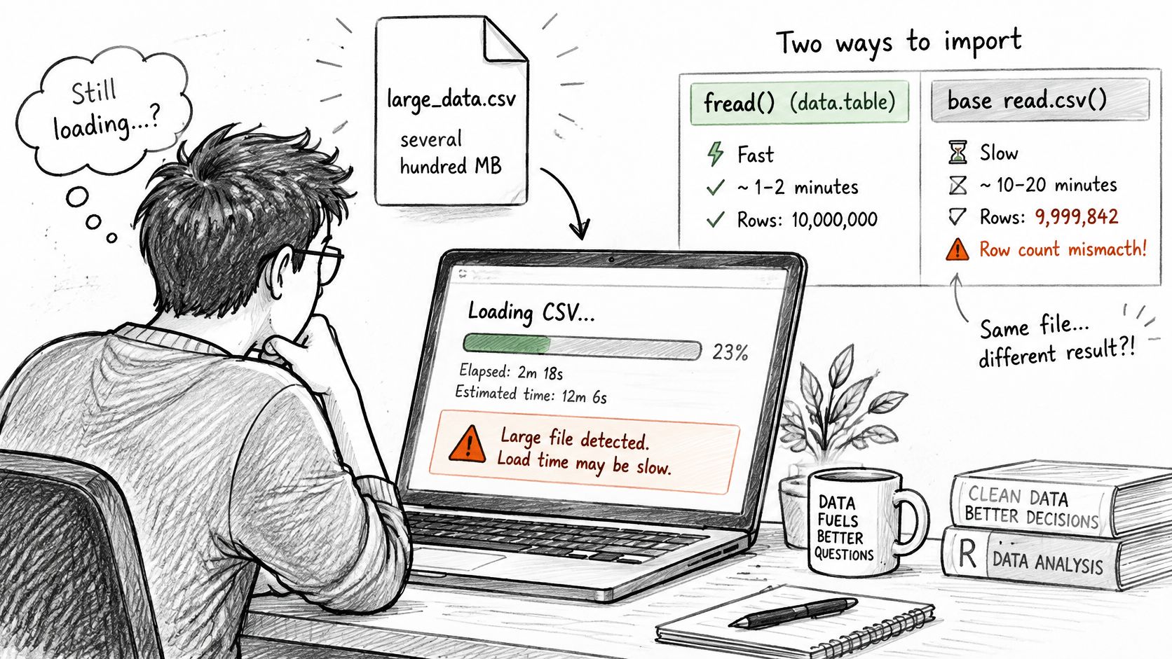
Choose by what you need, not by habit. fread() gives speed and automatic detection. read_csv() gives typed columns and warnings. read.csv() with colClasses cuts conversion work and memory, and the base R read.table help page supports setting classes directly, including colClasses = "character" for a lossless staging import.

Stage as character, then convert deliberately

Read everything as character with colClasses = "character" or col_character(), validate row counts and missing value counts against the source, then convert named columns explicitly. You pay one controlled conversion instead of debugging a dozen guessed ones.

Benchmark rule: Time the complete workflow, including transformations, joins and output. Timing only the read misleads, because character values enter R's global string cache and later steps pay costs the timer missed.

Record elapsed time, peak memory, row count agreement, column classes, missing value counts and parse error counts for each run, on representative files rather than clean synthetic ones. Watch for memory pressure from wide character staging, repeated conversions when a later join needs the same column, and benchmark runs that differ only because their inputs differed.

Finish by storing a checksum of the raw file from tools::md5sum() next to the exact import specification. An audit can then show the same bytes produced the same result.

Confirm the Import Before You Analyze Anything

A sales_q3.csv can enter your session with no warning and still be wrong. A quoted line break shifts every later row. An identifier that should keep a leading zero arrives as an integer. An accented name comes through garbled. Before any model or summary, prove the object in memory is the file you meant to load.

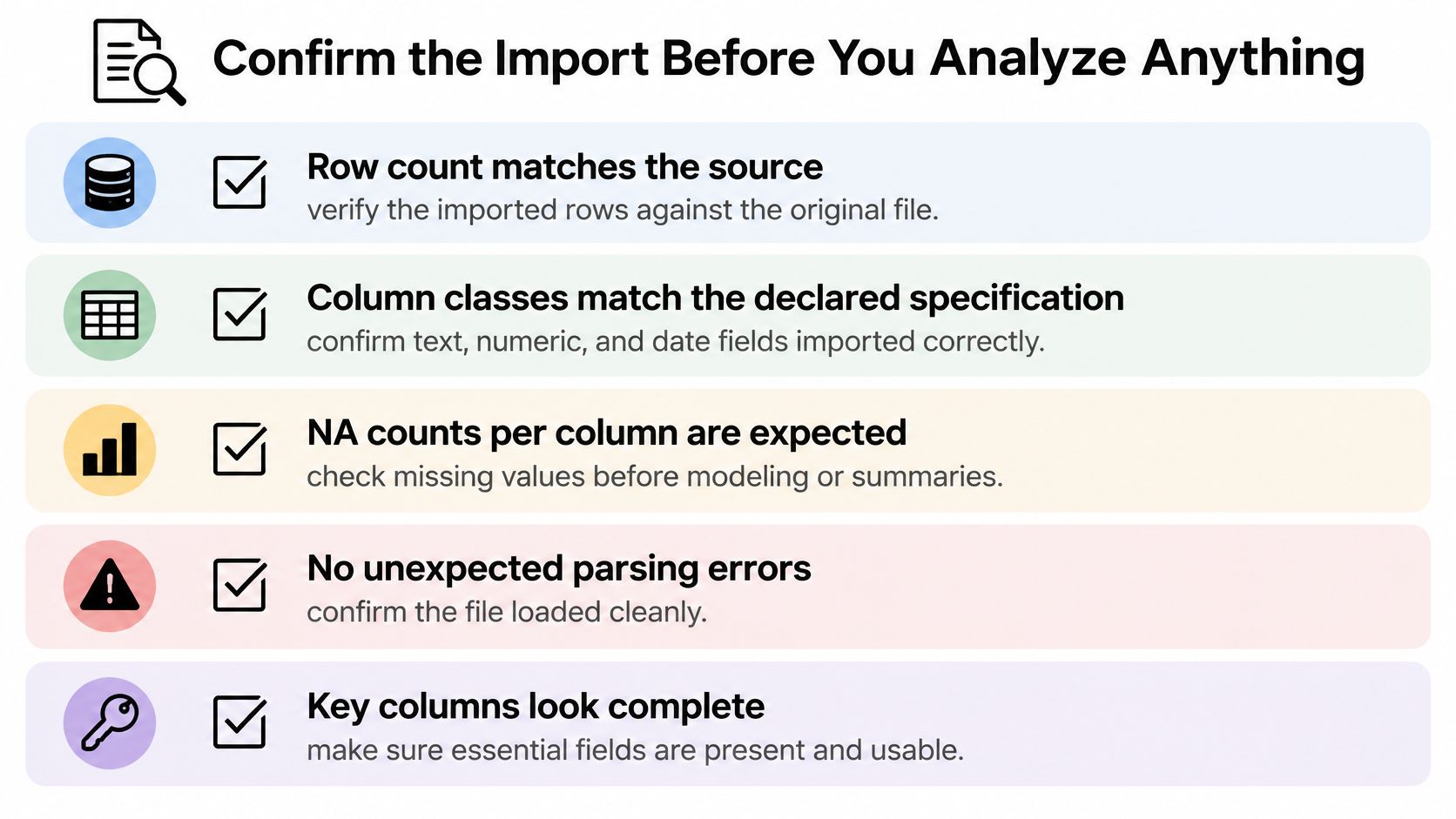
Run these checks on the imported object:

• Row count matches the source record count exactly.
• Column classes match your declared specification.
• NA counts per column are plausible and match your missing code list.
• One known record checks out, including a leading zero identifier and an accented name.
• Dates are Date values, not text that merely looks like dates.
• problems() returns nothing unexpected on readr imports.

If any check fails, correct the import specification and reload. Leave the analysis alone until the object matches the source. Save the import script with the specification, encoding, and checksum so a rerun produces the same result.

As a second look at that same file, PlotStudio AI supports common formats such as CSV and Excel tables, processes data files locally on your machine without uploading them to its servers, and can inspect a dataset while running Python locally. Those checks still apply to whatever it receives. Its AI for CSV analysis starts from that verified file.

Take your next verified sales_q3.csv, open it in PlotStudio AI alongside your R script, and compare the profile against your checklist before you model anything.