The common advice to use Spearman whenever data aren't normal is incomplete. Spearman correlation analysis measures monotonic association, whether higher values tend to accompany higher or lower values, using ranks rather than raw measurements. A defensible analysis starts with the relationship's shape and the observations' structure, then checks whether ties and missing data make the p-value and confidence interval trustworthy.
What Spearman Correlation Measures and When to Use It
Spearman's rho describes how consistently observations maintain the same ordering across two variables. It captures relationships that generally move in one direction, even when the rate of change isn't constant.
The coefficient ranges from −1 to +1: a perfectly increasing rank relationship gives +1, a perfectly decreasing relationship gives −1, and zero indicates no rank association, as the NIST rank-correlation reference explains. The distinction is between association in the ordering of observations and association in their original measurement units.
Say a clinic investigates waiting time and satisfaction ratings. Spearman asks whether patients who wait longer generally rank lower in satisfaction. It doesn't assume that the difference between adjacent satisfaction categories represents an equal change in experience.
Pearson, Spearman and Kendall compared
| Measure | What it captures | Data it suits | Ties and outliers |
|---|---|---|---|
| Pearson r | Linear association between raw values | Interval or ratio data; conventional inference often assumes approximate bivariate normality | Outliers can dominate the result |
| Spearman rho | Monotonic association between ranks | Ordinal, skewed or continuous data | Ties get average ranks; extreme magnitudes become ordinary ranks |
| Kendall tau-b | Agreement in the ordering of all pairs | Ordinal data with many ties | Tie-corrected; values are usually smaller in magnitude than rho |
The coefficients answer related but different questions. Kendall tau-b summarizes concordance and discordance between pairs, whereas Spearman measures correlation between ranked variables. Don't select whichever produces the smallest p-value.
Why ranks help with extreme observations
An unusually long waiting time may be far beyond every other observation numerically, but ranking places it at the end of the ordering. Its numerical distance from the other values no longer directly determines its influence.
In a 2024 simulation study, de Winter, Gosling and Potter compared sample sizes from 5 to 1,000 and found that choosing Spearman rather than Pearson could reduce standard-deviation variability by about 20% in heavy-tailed data, according to their simulation paper. That's a finding about those simulated conditions, not a guarantee for every skewed dataset.
Selection rule: Choose the association you want to estimate before choosing the test that calculates it.
Start with Spearman for ordinal measurements or a research question about monotonic ordering, particularly when extreme magnitudes would distort a raw-value summary. Choose Pearson when the question concerns linear association between quantitative measurements. A nonnormal histogram alone doesn't disqualify Pearson; inspect the scatterplot and the inferential assumptions too.
For the broader distinction between describing association and testing it, the guide to correlation analysis provides useful context.
How to Run Spearman Correlation in Python and R
The computational command is short. Most consequential decisions happen before you run it: defining an observation, coding ordinal categories, and deciding which rows belong in the analysis.
For a clinical dataset, establish whether each row represents a patient or a visit. Treating repeated visits as independent patients produces an inferential problem that ranking won't fix.
A reproducible sequence
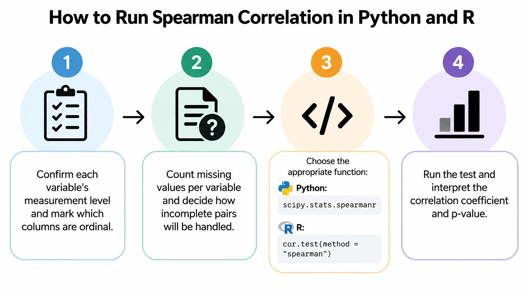
Confirm measurement levels. Mark ordinal columns and verify that their codes preserve the intended order. Convert labels such as mild, moderate and severe using an explicit ordering, not alphabetical sorting.
Count missing values separately for each variable, then identify complete pairs. Choose the missing-data policy before testing, and retain participant identifiers so exclusions can be audited.
Create average ranks. In pandas, use
rank(method='average')for each variable. Keep both the original-value scatterplot and the rank plot because they reveal different aspects of the measurements.Plot ranks against ranks and add a smoother. In Python, use
plt.scatter(x.rank(method='average'), y.rank(method='average'))andstatsmodels.api.nonparametric.lowess; in R, useplot(rank(x), rank(y))followed bylines(lowess(rank(x), rank(y))). Save the resulting figure as the candidate Figure 1.Calculate the coefficient and p-value. Python's
scipy.stats.spearmanr(x, y)returnsstatisticandpvalue. R'scor.test(x, y, method='spearman')returns the estimate and test result, with a warning when ties prevent its usual exact calculation.For a wider exploratory analysis, construct a correlation matrix. Select only analytically meaningful numeric columns, excluding identifiers and numeric codes for unordered categories.
Add an interval and preserve the run. Save the resampling procedure, random seed, package versions, input-file version and figure. A coefficient without its analysis settings is difficult to reproduce reliably.
The process graphic summarizes the main decisions before interpretation.
Minimal Python and R examples
These examples assume a CSV containing waiting_time and satisfaction. They deliberately use the same complete pairs for the coefficient, test and reported sample size.
Python
import pandas as pd
from scipy.stats import spearmanr

df = pd.read_csv("clinic.csv")
pair = df[["waiting_time", "satisfaction"]].dropna()
x, y = pair["waiting_time"], pair["satisfaction"]
result = spearmanr(x, y)
print({"rho": result.statistic,
       "p_value": result.pvalue,
       "n": len(pair)})
R
df = read.csv("clinic.csv")
pair = na.omit(df[c("waiting_time", "satisfaction")])
result = cor.test(pair$waiting_time, pair$satisfaction,
                  method = "spearman")
print(list(rho = unname(result$estimate),
           p_value = result$p.value,
           n = nrow(pair)))
Don't silence the R ties warning without understanding it. Setting exact=FALSE makes the approximate calculation explicit; it doesn't improve its accuracy automatically.
Spearman functions in Python and R
| Task | Python (SciPy, pandas) | R (stats, boot) | Returns |
|---|---|---|---|
| Pairwise rho and p-value | scipy.stats.spearmanr(x, y) |
cor.test(x, y, method='spearman') |
Rho and p-value |
| Correlation matrix | df.corr(method='spearman') |
cor(df, method='spearman') |
Rho for every pair, no p-values |
| Missing pairs | df.corr(method='spearman') with pairwise NaN handling |
cor(df, method='spearman', use='pairwise.complete.obs') |
Pairwise rho; calculate pair-specific n separately |
| Bootstrap BCa interval | scipy.stats.bootstrap with paired=True, method='BCa' and a Spearman statistic |
boot() with boot.ci(type='bca') |
Confidence interval at the chosen confidence level |
A successful run has a coefficient whose sign matches the plotted direction, an n matching the eligible pair count, and a clearly identified p-value method. If either variable is constant, stop: its correlation is undefined.
Handling Ties, Missing Data and Nonmonotonic Patterns
The first trap is treating tied categories as distinct positions. Say a hypothetical five-category satisfaction item has most responses concentrated in its highest categories. Respondents selecting the same category receive the average of the ranks their observations occupy, not an arbitrary ordering within that category.
The illustration shows how tied responses translate into average ranks.
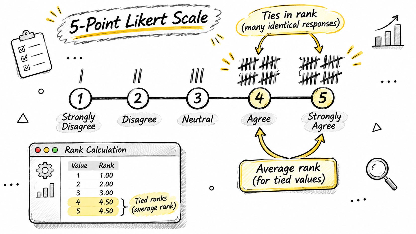
The formula trap is applying the distinct-rank shortcut to tied data. The familiar expression, rho = 1 − 6Σd²/[n(n² − 1)], assumes no ties; software instead computes Pearson correlation between average ranks when ties occur. Calculate ranks within the actual complete-pair sample, rather than ranking an entire column and then discarding incomplete observations.
Missingness changes the analysis sample
The deletion trap is assuming every matrix cell describes the same participants. Listwise deletion uses rows complete across all selected variables, while pairwise deletion uses the available rows for each relationship. Record n per pair and check whether different coefficients describe meaningfully different subsets.
The imputation trap is replacing missing responses with a mean before ranking. That creates an artificial concentration of equal values and can distort the association. When a missing-at-random assumption is defensible, consider multiple imputation with models appropriate to ordinal variables and a justified pooling procedure; observed missingness patterns can inform, but can't prove, that assumption.
The guide to handling missing data helps distinguish a convenient deletion rule from a defensible missingness strategy.
A near-zero coefficient can hide structure
The shape trap is confusing no monotonic association with no dependence. A direction-changing relationship can produce a near-zero coefficient despite a clear pattern, a limitation discussed in this educational article on correlation methods.
Compare two illustrative simulation designs: independent variables produce a shapeless cloud, while a symmetric U-shaped response falls and then rises. Both can yield a near-zero rho, but their scientific interpretations are entirely different.
A near-zero rho is a reason to inspect shape, not permission to declare independence.
Use a rank scatterplot with a LOWESS or LOESS smoother, and examine regions of the predictor without selecting splits merely to manufacture significance. Consider spline regression or segmented regression when the curve itself matters, and distance correlation or mutual information when broader dependence is the target.
This video offers an additional explanation of rank correlation.
A nonsignificant result means insufficient evidence against the tested null under the chosen procedure. It doesn't establish independence.
Testing Significance and Building Confidence Intervals
A p-value is trustworthy only to the extent that its reference distribution matches the data and design. Independent observations, the amount of tying, sample size and the chosen null hypothesis all matter. Calling a method nonparametric doesn't remove those requirements.
For testing a zero population rank correlation, a common large-sample approximation uses:
t = rho × √[(n − 2)/(1 − rho²)]
This is an approximation for Spearman inference, not an exact small-sample guarantee. It's more defensible with sufficiently large continuous samples than with sparse, heavily tied ordinal responses.
Match inference to measurement resolution
A 2025 simulation preprint on Spearman confidence intervals found good analytic-interval coverage with continuous data but poorer coverage with ordinal data; BCa bootstrap intervals performed well at moderate sample sizes such as N ≥ 50 with about 2,000 resamples. Treat those settings as evidence from the studied conditions, not a universal minimum.
Inference methods for Spearman rho
| Method | Output | Best for | Watch for |
|---|---|---|---|
| Analytic t-based test | Approximate p-value; interval requires a separate approximation | Continuous data with few ties and adequate sample size | Interval coverage can weaken with ordinal data |
| Bootstrap BCa | Confidence interval | Ordinal data with adequate sample size and nondegenerate resamples | Sparse categories can create undefined bootstrap correlations |
| Permutation test | P-value from a shuffled null distribution | Small samples or heavy ties under exchangeability | Monte Carlo stability and the precise null being tested |
| Kendall tau-b with bootstrap | Sensitivity interval | Checking conclusions under heavy ties | Different scale; compare conclusions rather than raw values |
A t-based test doesn't automatically provide a well-calibrated interval for rho. Keep the test method and interval method separate in your code and reporting.
Resample the correct unit
For a paired bootstrap, sample complete rows with replacement, recompute rho after reranking each sample, and construct percentile or BCa-adjusted limits. Never resample the two columns independently, because that destroys the relationship you're estimating.
For a permutation test, shuffle one variable relative to the other and compare the observed statistic with the shuffled distribution. This requires exchangeability and typically tests an independence-based null, which is stronger than merely asserting zero population rho. Clustered or repeated observations require design-aware resampling.
Before accepting an interval, inspect:
- Unique levels and ties. Count observed categories and the concentration within them.
- Degenerate resamples. Identify bootstrap samples in which a variable becomes constant.
- Sensitivity. Compare the substantive conclusion with Kendall tau-b or an appropriately specified ordinal model.
Large samples can make small associations statistically detectable. Evaluate the estimate's practical meaning and interval width, not just whether the p-value crosses a threshold.
The explanation of confidence intervals clarifies how interval uncertainty differs from the probability that a particular hypothesis is true.
Comparing Two Correlations and Planning Sample Size
A significant correlation in one group and a nonsignificant one in another does not, by itself, show that the groups differ. Estimate the difference between their correlations directly, choosing a method that reflects whether observations are independent or shared.
For treatment and control groups, calculate rho in each arm, then bootstrap the difference by resampling participants within each arm. Avoid applying Pearson's Fisher transformation and its usual standard error automatically to Spearman coefficients.
Independent groups versus shared participants
| Comparison | Resampling approach | Important restriction |
|---|---|---|
| Separate treatment and control groups | Resample within groups and calculate the difference in rhos | Preserve group membership and sampling structure |
| Correlations measured on the same people | Resample whole participant rows and calculate both correlations | Preserve shared variables and within-person dependence |
| Group-label permutation | Shuffle labels under a justified exchangeable null | Equal correlations alone don't guarantee exchangeable groups |
Group-label permutation is useful only when its null matches the scientific question. If groups have different marginal distributions, their labels are not automatically interchangeable, even when the correlations may be equal.
For repeated player appearances, preserve the player-level structure rather than treating every appearance as independent. The FPL Player Stats comparison research offers a sports-statistics context for comparisons involving player data.
Plan for precision, not just significance
A 2024 methodological study in the Journal of Clinical and Translational Research reported sample-size requirements from 86 participants for an expected correlation of 0.9 to 1,331 for an expected correlation of 0.3, under its planning conditions for a 95% confidence interval. These figures depend on those conditions. A confidence level alone cannot determine sample size; the desired precision matters too.
Weaker expected associations can require substantial recruitment when the goal is a precise estimate. Use prior literature or a cautiously interpreted pilot estimate, and specify the expected rho before collecting the main dataset.
Set out the remaining planning choices:
- Precision target. Define the acceptable interval width.
- Measurement resolution. Anticipate category frequencies and ties. Many tied ranks can affect how informative the estimate and its uncertainty are.
- Attrition allowance. Account for dropout and incomplete pairs.
- Testing family. Define which correlations will be included in a Benjamini-Hochberg false-discovery-rate adjustment.
Tools covered in the power-analysis software guide can support planning. Choose a calculation that matches the quantity being estimated and the intended inference. A near-zero rho is not proof of independence: inspect the pattern and tie structure, and consider whether the study was designed to estimate a sufficiently precise interval.
Reporting Spearman Results and Next Steps
A near-zero Spearman coefficient does not prove that two variables are independent. It says their ranked values show little overall monotonic association. A curved or otherwise nonmonotonic pattern can still be present, and tied ordinal responses can affect how much confidence to place in the p-value and interval. Report the statistic alongside a plot and enough detail for readers to assess those limits.
A concise format is rₛ = value, n = sample size, p = value, confidence interval [lower, upper]. Define n as the number of complete pairs used. Avoid placing sample size in parentheses after the coefficient unless the notation makes its meaning clear.
For a hypothetical reporting example, not an observed finding: rₛ = .62, n = 48, p < .001, 95% CI [.41, .77]. The estimate describes ranked association, while the interval and p-value summarize uncertainty under their respective procedures.
A manuscript-ready template
Spearman rank correlation assessed the association between [variable A] and [variable B] because [measurement or relationship rationale]. Ties received average ranks, and [missing-data policy] yielded [n] complete pairs. The association was [direction], rₛ = [estimate], p = [value], with a [confidence level] BCa bootstrap interval [lower, upper]. Figure 1 displays the rank-versus-rank scatterplot and smoother.
In the methods, state the bootstrap resample count, random seed, software and package versions. Describe the p-value procedure separately from the bootstrap interval; they are distinct inferential choices. If ties are heavy, report a Kendall tau-b sensitivity result in a supplementary note and say whether it changes the interpretation.
Spearman reporting elements
| Element | What to write | Example |
|---|---|---|
| Coefficient and n | rₛ and the number of complete pairs | Hypothetical rₛ = .62, n = 48 |
| Significance | P-value or an appropriate threshold | Hypothetical p < .001 |
| Interval | Confidence level and method | Hypothetical 95% BCa CI [.41, .77] |
| Ties and missing data | Handling rule and pair count | Average ranks; pair-specific complete-pair counts |
| Plot reference | Figure showing ranked values | Figure 1 shows the rank-versus-rank scatterplot |
| Sensitivity | Alternative coefficient and conclusion | Kendall tau-b when ties are heavy |
Describe variables as associated, not as causing one another. An unadjusted rank correlation does not account for age, baseline severity, socioeconomic circumstances or other confounders.
For exploratory correlation matrices, separate hypothesis generation from prespecified confirmatory testing. Name the multiple-testing correction and report adjusted results transparently, rather than showing only favorable cells. The methods-section writing guide can help structure a reproducible account of these analytical decisions.
Common questions about Spearman correlation analysis
Does Spearman correlation require normally distributed data?
No. Its rank-based calculation does not require normally distributed raw variables. The sampling design and inferential procedure still need justification.
Can I use Spearman with Likert responses?
Yes, when the categories have a meaningful order. Report observed category frequencies, since coarse measurement creates ties that can affect uncertainty estimates.
Can I square Spearman rho to report variance explained?
Not as a proportion of variance explained in the original measurements. Rho summarizes ranked association, so squaring it would imply a different interpretation.
How should I validate an AI-generated Spearman analysis?
Use a dataset with a known result and check the eligible rows, ranks, coefficient, inference settings and figure. A plausible narrative alone is not validation.
Where agentic analytics helps
Agentic analytics is data analysis performed by AI agents that can plan an investigation, execute analytical steps with real tools and code, inspect intermediate results, revise the approach, validate outputs, and synthesize a complete analysis. An answer is an output; an analysis is an investigation.
PlotStudio AI is a desktop application for agentic data analytics. Users upload a dataset and ask questions in plain English; specialized AI agents plan, code, execute and narrate multi-step analyses locally on the user's machine. Each question produces a permanent Analysis Page containing tables, charts, statistical tests and interpretation. Researchers should still assess whether the scientific rationale and outputs fit their question.
Try PlotStudio AI at https://www.plotstudio.ai/ with a dataset whose result you already know. Compare the ranks, pair counts, interval settings and saved analysis with the expected result.