You've fitted a regression to ordered observations, and the coefficient looks stable, but the p-value suddenly becomes much smaller after a software update. Or your forecast errors look unnaturally smooth across time. Autocorrelation may be the reason. It measures how a variable, residual, or error relates to its own lagged values, and it matters because dependence changes how much independent information your data really contains.
A Direct Answer for Curious Analysts
Autocorrelation is the correlation between a variable and an earlier version of itself. If (X_t) is the value observed now, autocorrelation asks whether (X_t) is related to (X_{t-k}), the value observed at lag (k). The same idea applies to a raw outcome series, regression residuals, or an unobserved error process.
Suppose a demand forecaster's errors are positive for several periods and then negative for several periods. The model may be missing a trend, seasonal pattern, delayed effect, or other time-dependent structure. Alternatively, a panel regression may produce nearly identical coefficients after a change in software, while the standard errors and p-values shift noticeably. The coefficient didn't necessarily become more informative. The estimated uncertainty changed because the observations weren't independent.
A useful distinction is often missed in beginner explanations. Autocorrelation isn't automatically a problem, and its main damage may be inferential rather than point-estimate bias. Under suitable exogeneity conditions, autocorrelated regression errors can leave coefficient estimates unbiased while making conventional standard errors unreliable. Positive serial correlation commonly makes those standard errors too small, which can inflate test statistics and make confidence intervals look more precise than they should. The CASRAI guide to autocorrelation in time-series data presents this distinction and connects the problem to the amount of independent information in a sample.
Practical rule: Don't ask only whether autocorrelation exists. Ask what quantity you're trying to estimate.
The diagnostic path is therefore straightforward. First, identify where dependence appears. Next, check whether the series is stationary or merely trending. Then decide whether autocorrelation is a nuisance for inference or the dynamic structure you want to model. A standard error that tolerates heteroskedasticity may be enough for the first problem. The second may require an explicit time-series, mixed-effects, state-space, or lagged-error model.
If you're starting with the broader idea of association, this guide to what correlation analysis means provides useful groundwork. Autocorrelation is a special case, but the ordering of observations creates the important difference.
What Autocorrelation Actually Means
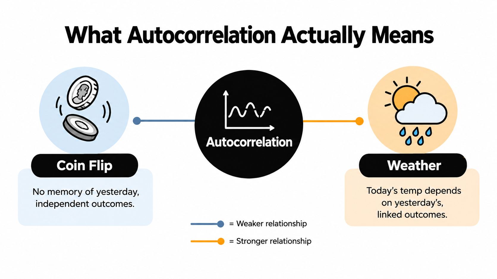
Start with two familiar examples. A fair coin flip has no memory of the previous flip. Knowing yesterday's result doesn't help you predict today's result, so successive outcomes are independent in the idealized model. Weather behaves differently. Today's temperature is partly related to yesterday's because the atmospheric state changes gradually rather than resetting between observations.
That is the intuition behind positive autocorrelation. Nearby values tend to be similar, so a high value is often followed by another high value and a low value by another low value. Negative autocorrelation produces alternation. A high value tends to be followed by a low value, or a positive residual by a negative residual. The pattern can weaken as the lag grows, which is often described as geometric decay.
The formal definition
At lag (k), the population autocorrelation is commonly written as:
[
\rho_k =
\frac{\operatorname{Cov}(X_t, X_{t-k})}
{\sqrt{\operatorname{Var}(X_t)\operatorname{Var}(X_{t-k})}}
]
The sample version replaces population moments with quantities calculated from observed data. Like an ordinary correlation coefficient, autocorrelation lies between (-1) and (1). A value near zero means little linear association at that lag, although it doesn't prove that no nonlinear or conditional dependence exists.
A useful correlation definition can help clarify the common structure. Autocorrelation uses the same variable twice, but one copy is shifted in time. That shift is what makes the relationship about memory rather than mere association between two different measurements.
Three places dependence can appear
The outcome series itself. Sales, temperature, patient measurements, financial returns, or sensor readings may show persistence, seasonality, or another time-dependent pattern.
Regression residuals. A regression may explain the average relationship while leaving time structure in the unexplained part. This is especially important because ordinary least squares commonly relies on independent errors for conventional inference.
The structural error process. In a time-series model, the dependence may be an explicit part of the data-generating process. An autoregressive error model, for example, treats today's unexplained component as related to earlier unexplained components.
Weak autocorrelation can still matter when the dataset contains many observations. A long sequence of nearby measurements may look large on paper while containing much less independent information than the same number of unrelated observations. That's why analysts should interpret autocorrelation in relation to the sampling process, not by looking at the coefficient alone.
Reading ACF and PACF Without Misreading Them
The autocorrelation function, or ACF, reports the correlation between a series and lagged versions of itself across several lags. It captures both direct and indirect pathways. If the current value relates to the previous value, and the previous value relates to an earlier value, the ACF can reflect that chain even when the current value has no direct relationship with the more distant observation.
The partial autocorrelation function, or PACF, asks a narrower question. It measures the association at a given lag after accounting for the intermediate lags. Analysts often estimate it through successive regression relationships or equivalent recursive procedures. The ACF shows total dependence, while the PACF is closer to the remaining direct dependence at each lag.
A practical pattern guide
| Process | ACF pattern | PACF pattern | Recommended response |
|---|---|---|---|
| Autoregressive structure | Gradual decay is common | A clearer cutoff may identify the relevant lag depth | Consider an autoregressive specification, then check residuals |
| Moving-average structure | A cutoff may appear after the relevant lag depth | Gradual decay is common | Consider a moving-average specification and validate the residuals |
| Mixed autoregressive and moving-average structure | Gradual decay may occur | Gradual decay may also occur | Compare plausible models using diagnostics and domain knowledge |
| Trend or nonstationary process | Slow decay across many lags | Persistent patterns can also appear | Inspect stationarity, plot the series, and consider differencing or a long-run model |
These patterns are clues, not automatic identification rules. ACF and PACF plots can be distorted by finite samples, missing observations, structural breaks, seasonality, and an unsuitable mean specification. A seasonal process may produce repeated spikes at the seasonal spacing, but a trend can create broad persistence that resembles a strong autoregressive process.
The nonstationarity trap
A trending or unit-root series can produce a slowly declining ACF and an apparently impressive regression with another trending series. The apparent relationship may be driven by shared movement through time rather than a meaningful connection. The university course material on autocorrelated series warns that nonstationarity can generate autocorrelation, misleadingly strong fits, and inappropriate significance tests.
A high ACF is evidence of persistence in the observed series, not automatically evidence of a causal mechanism.
A sensible workflow plots the data before interpreting the correlogram. It checks stationarity, examines residuals, considers known breaks, and asks whether differencing would remove signal that matters scientifically. Differencing can help with a unit-root-like process, but it can also remove long-run equilibrium information. When several nonstationary variables share such an equilibrium, cointegration methods may be more appropriate.
For a broader overview of methods and model choices, see time-series analysis methods. The practical lesson is simple: use ACF and PACF to generate hypotheses about structure, then test those hypotheses against the research design and residual behavior.
Statistical Tests for Serial Dependence
A plot is often the best first diagnostic, but formal tests help document the evidence. No single test detects every form of serial dependence. Each has a null hypothesis, a target pattern, and boundary cases where its result can mislead.
| Test | Null hypothesis | Detects | Misses or limits | Typical use |
|---|---|---|---|---|
| Durbin–Watson | No first-order residual autocorrelation | Linear dependence between neighboring regression residuals | Higher-order dependence and models with lagged dependent variables | A quick residual diagnostic after regression |
| Breusch–Godfrey | No serial correlation through the selected lag order | Higher-order autoregressive residual dependence and dynamic regressors | Results depend on the chosen lag order and model specification | A more flexible regression residual test |
| Ljung–Box | Residual autocorrelations are jointly zero through the selected horizon | Cumulative evidence across several residual lags | It should diagnose fitted residuals, not be applied casually to raw trending data | Checking whether residuals are approximately white |
| Runs test | The sequence of signs is consistent with randomness | Some sign patterns, drift, and alternation | It ignores magnitude and may have limited power for other forms of dependence | A nonparametric complement to correlation-based tests |
Durbin–Watson is narrow by design
The Durbin–Watson statistic is mainly a first-order diagnostic. It is useful when the concern is adjacent residuals in a regression without lagged dependent variables. It becomes difficult to interpret when the model includes lagged regressors, particularly a lagged outcome. In that setting, Breusch–Godfrey is usually the more suitable regression test.
An analyst might report: “Residual first-order serial dependence was assessed with the Durbin–Watson statistic.” That sentence is transparent because it doesn't claim the test examined every possible lag.
Breusch–Godfrey asks a broader regression question
Breusch–Godfrey is a Lagrange multiplier test based on an auxiliary regression of residuals on the original regressors and lagged residuals. The analyst chooses the maximum lag order in advance or justifies it using the sampling frequency and substantive process. The report should state that lag order and explain whether the test rejected the null of no serial correlation through that order.
Ljung–Box evaluates residual whiteness
The Ljung–Box test aggregates information from several residual autocorrelations. It's particularly useful after fitting an ARIMA-like model, where the central question is whether the remaining errors resemble white noise. Applying it directly to raw data can confuse predictable trend or seasonality with model failure. The test's result only makes sense relative to the fitted model and the lag horizon selected.
The runs test uses signs rather than magnitudes. That makes it a useful complement, especially when the sequence alternates or drifts in a way that a linear correlation summary doesn't capture. It isn't a replacement for residual plots, stationarity checks, or a model-based diagnostic.
For choosing among statistical procedures more generally, statistical test selection can help frame the question around the estimand, design, and assumptions rather than around whichever test happens to be available in the software menu.
Matching the Remedy to the Estimand
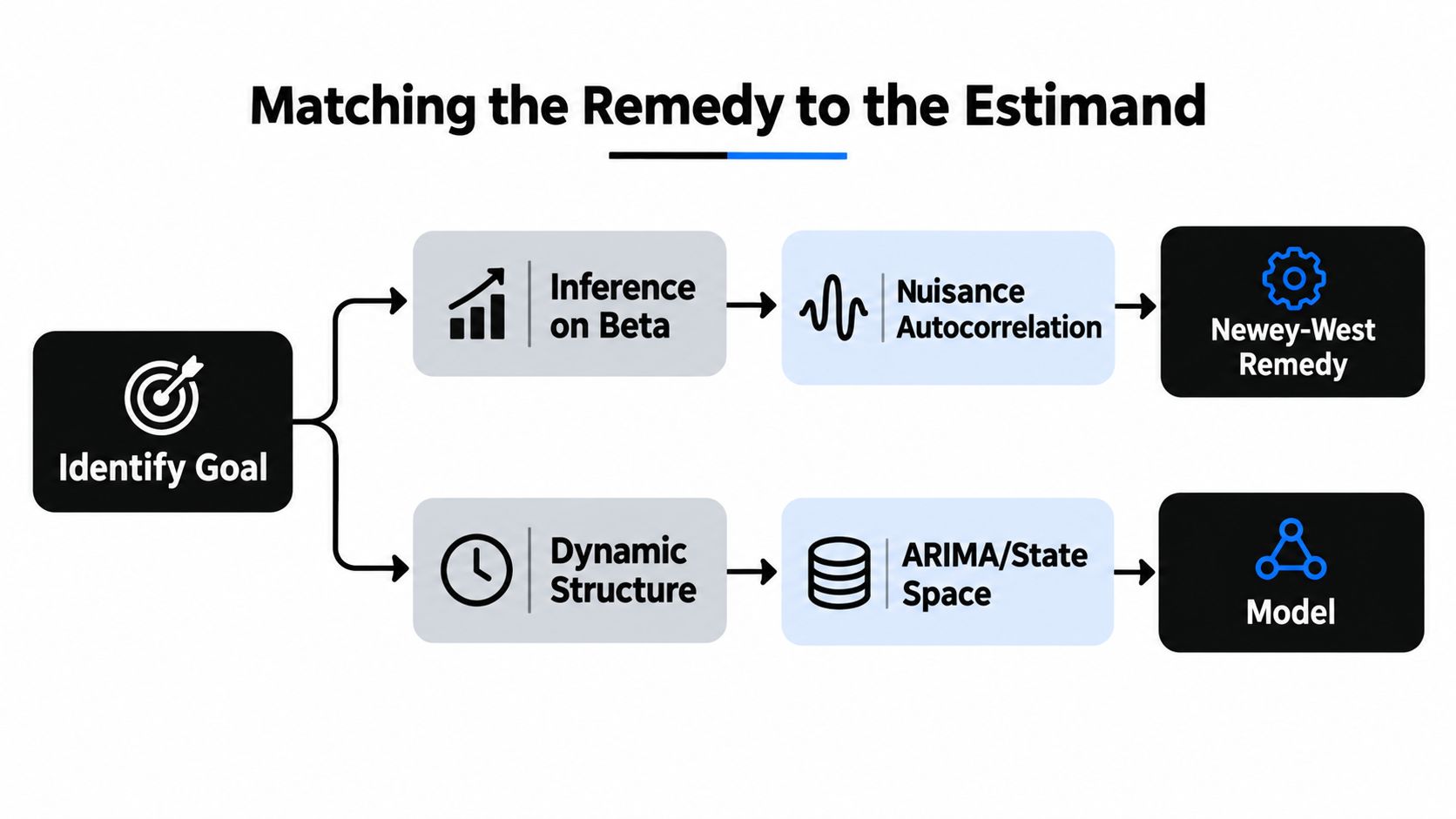
The key decision is not “Which autocorrelation correction should I use?” It is “What am I trying to estimate?”
If the target is a regression coefficient and the dependence is a nuisance, preserve the coefficient model and repair the inference. If the target is the dynamic structure itself, model the dependence directly. These are different estimands and shouldn't be treated as interchangeable.
When inference is the target
Newey–West or HAC standard errors change the estimated uncertainty around coefficients without changing the coefficient estimates themselves. They are useful when the regression specification is substantively appropriate and the main concern is valid tests and confidence intervals under serial dependence.
In panel data, cluster-robust standard errors can address arbitrary dependence within a defined cluster, provided the clustering structure matches the design. A panel researcher might cluster by individual, firm, region, or another unit that explains how observations can share shocks. The choice must follow the sampling and dependence structure, not convenience.
Estimand first: If you want the association conditional on the existing regressors, robust inference may be the right correction. If you want a dynamic forecast, it usually isn't enough.
The guide to robust standard errors is relevant when the coefficient is the object of interest and the model's errors are not independent.
When dependence is structural
Use GLS, Cochrane–Orcutt, Prais–Winsten, or feasible GLS when the covariance structure is part of the model and you want an estimator that uses it. These methods can improve efficiency when the error process is specified credibly, but a misspecified covariance model can produce a false sense of precision.
For forecasting, ARIMA errors with exogenous regressors can represent serial structure while preserving the influence of external predictors. The model should be judged through residual diagnostics and forecast validation, not merely by a visually attractive fitted line.
First differences can be appropriate for a series whose level is nonstationary. They may also destroy a meaningful long-run relationship. When nonstationary variables move together around an equilibrium, Engle–Granger approaches or a vector error-correction model can preserve that long-run information while modeling short-run changes.
Nested observations, repeated measures, and latent dynamics may call for mixed-effects models or state-space models. These approaches make the dependence structure explicit, but they still require decisions about random effects, measurement error, missingness, and validation.
The safest decision rule is to estimate the simplest model that answers the research question, then choose the estimator or standard error that matches the dependence present. Don't select a remedy because it is familiar. Select it because it preserves the quantity you need to interpret.
Two Worked Examples Analysts Can Reuse
A reproducible workflow should connect the diagnostic to the correction. The code matters, but so does the interpretation of what changes and what stays fixed.

Example one with a regression
Suppose a researcher models monthly retail sales using price and advertising expenditure. In Python, fit the model with statsmodels.api.OLS, then inspect the residuals over time. A residuals-versus-time plot can reveal runs, cycles, changing variance, or an unmodeled break that a single test statistic won't show.
Run the first-order diagnostic with statsmodels.stats.stattools.durbin_watson(results.resid). If the result suggests positive neighboring dependence, apply statsmodels.stats.diagnostic.acorr_breusch_godfrey(results, nlags=...) with a pre-specified lag order. The Breusch–Godfrey output includes a test statistic and a p-value. Interpret the p-value as evidence against the stated null for the selected lag structure, not as a probability that the model is correct.
If the research question concerns the price or advertising coefficient, refit the inference using results.get_robustcov_results(cov_type="HAC", maxlags=...). The coefficient estimates should remain the same under this correction, while the standard errors, test statistics, and confidence intervals can change. Report the original specification, the residual diagnostics, the HAC choice, and the fact that the inferential quantities were recalculated without changing the point estimates.
A report-ready interpretation could read: “The regression residuals showed evidence of serial dependence under the selected diagnostics. Because the estimands were the conditional associations between sales and the predictors, coefficients were retained and HAC standard errors were used for inference. The adjusted confidence intervals, rather than the conventional intervals, were used for interpretation.”
Example two with an autoregressive series
For a series whose dynamics are themselves the object of study, begin with a time plot and then call statsmodels.graphics.tsaplots.plot_acf(series) and plot_pacf(series). Read the two plots together. A slowly declining ACF with a more concentrated PACF pattern can support an autoregressive interpretation, but trend and nonstationarity must be ruled out first.
Fit the candidate model with statsmodels.tsa.arima.model.ARIMA(series, order=(p, d, q)).fit(). The order should come from the diagnostic reasoning, not from the visual pattern alone. Examine the fitted residuals with statsmodels.stats.diagnostic.acorr_ljungbox(fitted.resid, lags=..., return_df=True), then use the model's get_forecast() method to generate forecasts and intervals.
The Ljung–Box output asks whether residual autocorrelations through the selected horizon are jointly compatible with zero. If the residuals still show structure, revise the model, inspect breaks and seasonality, and validate forecasts using a time-ordered evaluation design. A good fit to the historical series isn't enough if the remaining errors are dependent or the forecast target has changed.
This is also where forecasting accuracy needs careful interpretation. Accuracy metrics can look favorable when a model benefits from temporal leakage, inappropriate random splitting, or an unexamined trend. The validation design must respect the order in which information becomes available.
The reusable principle is that regression inference and dynamic forecasting are not the same task. In the first example, the correction protects uncertainty around coefficients. In the second, the dependence is part of the forecast model and must be represented, tested, and validated.
Detection Workflow and the Autocorrelation FAQ
A practical diagnostic sequence can be short without being superficial.
Plot the series: Look for trend, seasonality, changing variance, gaps, outliers, and structural breaks.
Check stationarity: Use complementary diagnostics such as the augmented Dickey–Fuller and KPSS tests, while treating their assumptions and finite-sample behavior seriously.
Inspect ACF and PACF: Use them to identify persistence, possible seasonality, and candidate lag structures.
Test fitted residuals: Apply Ljung–Box to assess residual whiteness and Durbin–Watson when first-order regression residual dependence is the relevant question.
Choose the remedy: Use HAC or cluster-based inference when dependence is nuisance. Model dependence when forecasts or dynamic parameters are the target.
Refit and validate: Recheck residuals, confidence intervals, sensitivity to lag choices, missing-data decisions, and alternative specifications.
Common questions
Does correlation imply autocorrelation?
No. Ordinary correlation describes association between variables or measurements. Autocorrelation describes association between a variable and its own lagged values. A series can have cross-variable correlation without meaningful serial dependence, or serial dependence without the cross-variable relationship you expected.
Does a high ACF prove persistence?
No. A high ACF across many lags may reflect a trend or another nonstationary process. Plot the levels, inspect stationarity, and consider whether differencing or a long-run model is appropriate before interpreting the ACF as evidence of a durable mechanism.
Is Durbin–Watson enough?
No. Durbin–Watson is mainly a first-order diagnostic and has important limitations in regressions containing lagged dependent variables. Breusch–Godfrey can address higher-order dependence and dynamic regressors more directly.
Should I always difference the data?
No. Differencing may remove meaningful equilibrium information. If nonstationary variables share a stable long-run relationship, a cointegration framework may answer the research question more faithfully.
Agentic analytics can automate parts of this workflow by profiling a dataset, plotting ordered variables and residuals, running diagnostics, comparing a corrective change with the original model, and preserving the code and outputs for review. PlotStudio AI is one option for this kind of research data analysis. It can execute Python locally, produce charts and statistical tests, show the methodology and generated code, and save the result as a reproducible Analysis Page. The analyst still has to decide whether a detected pattern reflects the scientific process, a data-quality problem, a sampling artifact, or a modeling error.
Autocorrelation is therefore not a checkbox marked “detected” or “fixed.” It is a clue about dependence, information, and the estimand. The credible analysis is the one that explains where the dependence appears, why the chosen remedy fits the research question, and how the conclusions change under reasonable alternatives.
If you're analyzing sensitive research data, try PlotStudio AI's discounted academic plan, which includes 1,000 free credits for researchers while active. Use it to inspect your series, document the diagnostic decisions, and export a notebook or PDF that you can review before reporting the results.