The 2 sample t test formula divides the difference between two group means by the standard error of that difference: t = (x̄1 − x̄2) / SE. When you assume equal variances, SE is sp × √(1/n1 + 1/n2) and the degrees of freedom are n1 + n2 − 2. When you do not, SE is √(s1²/n1 + s2²/n2) and the degrees of freedom come from the Welch-Satterthwaite equation.
In plain terms, the formula asks how large the gap between two averages is compared with the noise you would expect from sampling alone. A large t means the gap is hard to explain by chance. A small t means it is not.
This article gives you both versions of the formula, defines every symbol, and walks one dataset through the full calculation by hand. You will also see how to read the result, which version to pick, and how to run the test in Excel, R, Python, or PlotStudio AI, where you can have the analysis written and executed for you and still check every step.
Why the two-sample t-test formula matters
What the formula tells you
The formula turns a raw gap between two averages into a signal-to-noise ratio. The numerator, x̄1 − x̄2, is the signal. The denominator, the standard error of the difference, is the noise you would expect from sampling alone. If the ratio is large, a gap that size would be rare when the two population means are actually equal.

Suppose a lab compares blood pressure reduction under a new regimen against a control. A 5.8 mmHg difference sounds meaningful, but with small groups and scattered readings it could easily appear by luck. The t statistic tells you how many standard errors apart the means are, and the degrees of freedom tell you how much to trust that count. Every two-sample version does this same job. They differ only in how they estimate the noise.
The t statistic is the difference between two means measured in standard errors, nothing more.
When the formula applies
Use it when you have two independent groups and one continuous outcome, such as a lab value, a score, or a time. Check these conditions before you calculate anything:
- Observations are independent, both within and between the groups.
- The outcome is continuous or close to it.
- Each group is roughly normal, or the samples are large enough that the means behave normally.
- For the pooled version only, the population variances are similar.
If the same people are measured twice, you need a paired t-test instead. With three or more groups, use ANOVA, because repeated pairwise t-tests inflate the false-positive rate. If a small sample is clearly skewed, a rank-based test such as the Wilcoxon rank-sum (Mann-Whitney) test is the safer choice.
The pooled and Welch formulas, term by term
The pooled formula for equal variances
The pooled version, often called Student's t-test, assumes both populations share one variance, so it blends the two sample variances into a single estimate before it builds the standard error.
sp² = ((n1 − 1) × s1² + (n2 − 1) × s2²) / (n1 + n2 − 2)
t   = (x̄1 − x̄2) / ( sp × √(1/n1 + 1/n2) )
df  = n1 + n2 − 2
The pooled variance is a weighted average of s1² and s2², weighted by each group's degrees of freedom, so the larger sample counts for more. The pooled SD always falls between s1 and s2. When n1 = n2 = n, sp² is simply the average of the two variances.
The Welch formula for unequal variances
Welch's version keeps the two variances separate. Nothing is pooled, which is why it holds up when group spreads or group sizes differ.
t  = (x̄1 − x̄2) / √(s1²/n1 + s2²/n2)
df = (s1²/n1 + s2²/n2)² / ( (s1²/n1)²/(n1 − 1) + (s2²/n2)²/(n2 − 1) )
The Welch-Satterthwaite degrees of freedom are rarely a whole number. They always land between the smaller of n1 − 1 and n2 − 1 and the pooled value n1 + n2 − 2. Software computes this for you, and you can use the fractional df as is.
What each symbol means
Every term in either formula comes from six quantities you can read off your summary statistics.
| Symbol | Meaning |
|---|---|
| x̄1, x̄2 | Sample mean of group 1 and group 2 |
| s1, s2 | Sample standard deviation of each group (s² is the variance) |
| n1, n2 | Number of observations in each group |
| sp | Pooled standard deviation, used only in the equal-variance version |
| SE | Standard error of the difference, the denominator of t |
| df | Degrees of freedom, which select the t distribution for critical values and p-values |
The null hypothesis is H0: μ1 = μ2, tested against Ha: μ1 ≠ μ2 for a two-tailed test. The Greek μ marks the unknown population means, while x̄ marks the sample means you actually measured.
Which version to use
Default to Welch. When variances and sample sizes are similar, it gives almost the same answer as the pooled test. When they differ, it keeps the false-positive rate near its nominal level, while the pooled test can drift, especially when the smaller group has the larger variance.
Use the pooled formula when you have a sound reason to assume equal variances, or when a protocol or course requires Student's test. Note that with equal group sizes the two t statistics are identical. Only the degrees of freedom differ.
Default to Welch's formula, and switch to the pooled one only when equal variances are an assumption you can defend.
How to apply the formula: a worked example
The data and the setup
These numbers are illustrative, chosen so the arithmetic is easy to follow. A trial measures the reduction in systolic blood pressure after eight weeks.
| Group | n | Mean reduction (mmHg) | SD |
|---|---|---|---|
| Treatment (group 1) | 12 | 12.0 | 4.0 |
| Control (group 2) | 15 | 6.2 | 8.0 |
We test H0: μ1 = μ2 against a two-tailed alternative at α = 0.05. Decide on α before you look at the results. The difference in means is 12.0 − 6.2 = 5.8 mmHg, and the SDs differ by a factor of two, so this is a good case to run both versions.
Calculating the pooled version
Work through the pooled formula in six steps:
- Pooled variance: (11 × 16 + 14 × 64) / 25 = 1072 / 25 = 42.88.
- Pooled SD: √42.88 = 6.548.
- Standard error: 6.548 × √(1/12 + 1/15) = 6.548 × √0.15 = 6.548 × 0.3873 = 2.536.
- Test statistic: t = 5.8 / 2.536 = 2.29.
- Degrees of freedom: 12 + 15 − 2 = 25.
- Critical value (two-tailed, α = 0.05, df = 25): 2.060. Because 2.29 is greater than 2.060, reject H0.
Calculating the Welch version
The Welch version skips the pooling and works from each group's variance divided by its sample size:
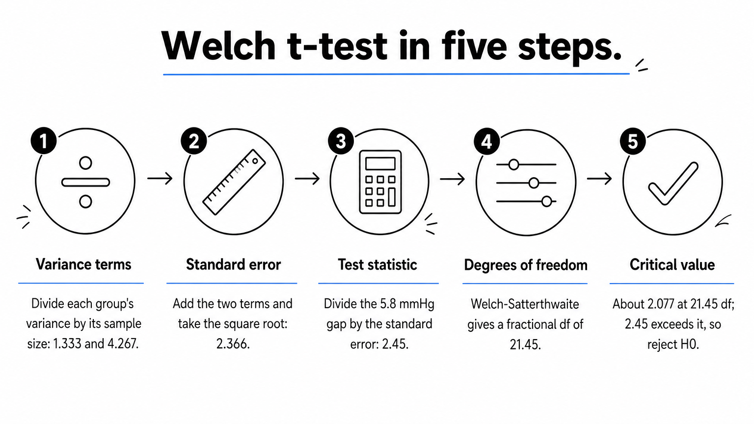
- Variance terms: 16 / 12 = 1.333 and 64 / 15 = 4.267.
- Standard error: √(1.333 + 4.267) = √5.600 = 2.366.
- Test statistic: t = 5.8 / 2.366 = 2.45.
- Degrees of freedom: 5.6² / (1.333² / 11 + 4.267² / 14) = 31.36 / (0.1616 + 1.3003) = 21.45.
- Critical value at about 21.45 df: roughly 2.077. Because 2.45 is greater than 2.077, reject H0.
Comparing the two results
| Quantity | Pooled | Welch |
|---|---|---|
| Standard error | 2.536 | 2.366 |
| t | 2.29 | 2.45 |
| df | 25 | 21.45 |
| Critical t (two-tailed, α = 0.05) | 2.060 | about 2.077 |
| Approximate p-value | about 0.03 | about 0.02 |
| Decision | Reject H0 | Reject H0 |
Both versions reject H0, but they disagree on the noise. The larger group has the larger variance here, so pooling lets that variance dominate and slightly overstates the standard error. If the smaller group had the larger variance, pooling would understate it and make the test too eager.
The two calculations differ only in how they estimate the noise, because the signal, 5.8 mmHg, is identical.
How to interpret the result and avoid mistakes
Reading t, critical values, and confidence intervals
Reject H0 when |t| exceeds the critical value for your df and α, or equivalently when the p-value falls below α. The critical value shrinks toward 1.960 as the degrees of freedom grow, so small samples need a larger t to reach significance.
| df | Two-tailed critical t (α = 0.05) | One-tailed critical t (α = 0.05) |
|---|---|---|
| 10 | 2.228 | 1.812 |
| 20 | 2.086 | 1.725 |
| 25 | 2.060 | 1.708 |
| 30 | 2.042 | 1.697 |
| 60 | 2.000 | 1.671 |
| Infinity | 1.960 | 1.645 |
Report more than a verdict. The 95% confidence interval for the difference is (x̄1 − x̄2) ± critical t × SE. For the pooled example that is 5.8 ± 2.060 × 2.536, or 0.58 to 11.02 mmHg. An effect size helps too: Cohen's d is the mean difference divided by sp, here 5.8 / 6.548, about 0.89. The wide interval is a useful reminder that a significant p-value can still leave the true effect poorly pinned down.
Mistakes that break the test
Most errors come from choosing the test badly, not from the arithmetic. Watch for these:
- Applying the test to paired data, such as before and after measurements on the same patients.
- Running several pairwise t-tests on three or more groups instead of one ANOVA.
- Choosing a one-tailed test after seeing which direction the data lean. The direction must be fixed in advance.
- Ignoring strong skew or outliers in small samples, where a rank-based test is safer.
- Treating statistical significance as proof of practical importance without looking at the interval and effect size.
How to run the test in software
Excel, R, and Python
You rarely compute the formula by hand, but you should know which version your software runs. The defaults differ, and that catches people out.

| Tool | Command | Note |
|---|---|---|
| Excel | =T.TEST(A2:A13, B2:B16, 2, 3) |
Type 2 is pooled, type 3 is Welch. Returns only the p-value. |
| R | t.test(x, y, var.equal = FALSE) |
Welch is the default. Set var.equal = TRUE for pooled. |
| Python | scipy.stats.ttest_ind(a, b, equal_var=False) |
Pooled is the default, so set equal_var=False for Welch. |
In Excel, the Data Analysis ToolPak offers "t-Test: Two-Sample Assuming Unequal Variances" and a pooled twin. Both show t, df, and the critical values. Whatever the tool, confirm the version from the output. Welch results show a fractional df.
Running it in PlotStudio AI
PlotStudio AI lets you upload a dataset, ask in plain English for a two-sample comparison, and specify Welch or pooled yourself. In Verification Mode you can review the proposed plan and its assumptions before anything runs. The analysis runs on your machine and produces a page with the test, a chart, and an interpretation.
You can inspect the generated Python, export the work as a Jupyter notebook, and check that its numbers match your hand calculation. The tool saves the typing, but you still own the judgment: whether the groups are independent, whether the assumptions hold, and what the result means for your study. You can try it free with 30 credits and no credit card.
Putting the formula to work
The two-sample t-test formula always has the same shape: a difference in means divided by a standard error. Pooled and Welch differ only in how they estimate that error, and Welch is the safer default. Check independence and normality first, compute t and the degrees of freedom, compare against the critical value, then report the interval and effect size alongside the p-value.
If you want to check your hand calculation against a real run, or skip the manual work on your next dataset, you can try PlotStudio AI free and review every step it takes.