Use an ANOVA test when you're comparing a numeric outcome across three or more groups or factor levels; for two groups, non-numeric outcomes, or incomplete repeated measurements, start with a t-test or a model suited to that structure. If you're staring at treatment labels and outcome columns, first decide which mean difference you want to estimate.
When an ANOVA Test Is the Right Test
ANOVA fits a question about population means, not a spreadsheet containing several groups. You need a numeric outcome, clearly defined factors, and a model that respects how observations were collected. The practical question is whether you want an overall comparison, a particular treatment contrast, or an estimate of change over time.
A factor is a categorical explanatory variable, such as treatment, genotype, or teaching method. Its levels are the categories being compared. A numeric code doesn't make an outcome continuous: coding disease status with digits still leaves you with a binary outcome.
Which test matches the comparison
| Data situation | Use this | Why this row |
|---|---|---|
| Numeric outcome, one factor, 3 or more independent groups | One-way ANOVA | One omnibus test of equal means |
| Numeric outcome, exactly two independent or paired groups | Two-sample or paired t-test | Equivalent ANOVA formulation gives F equal to t squared under the matching model |
| Two crossed factors, including their interaction | Two-way ANOVA | Separates main effects from dependence between factors |
| Same people at every level, complete and balanced | Repeated-measures ANOVA | Within-subject factor with no missing cells |
| Numeric outcome, independent groups, clearly unequal spreads | Welch ANOVA | Relaxes the equal-variance assumption |
| Binary, ordinal, or count outcome | GLM or ordinal model | Classical ANOVA targets means of a roughly continuous outcome |
| Repeated measures with missing visits or uneven times | Mixed-effects model | Doesn't require complete data or sphericity |
Read the table from the outcome and observation structure, not from the test name you recognize. Independent treatment groups suggest a between-subjects comparison. Measurements from the same participant require a paired or repeated structure, even if they occupy separate spreadsheet rows.
Crossed factors add another question. If you compare teaching methods across classroom settings, you may want to know whether a method's effect changes with the setting. That calls for an interaction, not merely a larger list of unrelated groups.
Unequal spreads and missing follow-up require different responses. Welch ANOVA addresses unequal group variances in an independent-group comparison. A mixed model addresses dependence and more flexible longitudinal structures; it isn't just another variance correction.
Write the estimand before choosing the test
The estimand is the quantity you want to learn about the population. Write it in ordinary language before translating it into software settings.
Practical rule: Complete the sentence, “I want to estimate the difference in average ___ between ___, accounting for ___.”
For example, you might want the difference in average yield between a candidate fertilizer and standard practice, accounting for field blocks. That sentence identifies an outcome, a specific comparison, and a design feature that the model must preserve.
Our statistical test selection guide provides a broader framework when your question doesn't fit a straightforward mean comparison.
A non-significant omnibus result doesn't establish practical equality. If the claim is that treatments are sufficiently similar for a clinical or operational purpose, define what sufficiently similar means and use an equivalence framework rather than interpreting absence of significance as proof.
What the F Statistic Is Comparing
Say you assign nitrogen rates to independent field plots and measure yield. Some plots outperform others because of soil variation, weather exposure, and measurement noise. The question is whether the differences between rate-specific averages are large relative to that plot-to-plot variation.
ANOVA compares those sources of spread using mean squares, which are sums of squared deviations divided by their associated degrees of freedom. For a simple one-way design:
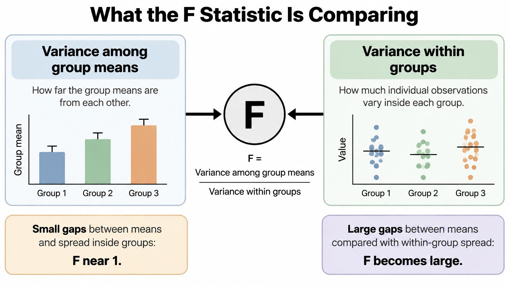
F = between-group mean square / within-group mean square
The numerator reflects how far group means sit from the overall mean, weighted by group size. The denominator estimates residual variation around each group's own mean.
The diagram separates the components of that ratio.
What a large F does and doesn't establish
Under the null hypothesis of equal population means, the mean squares estimate the same error variance, so their ratio tends to be near unity. A large ratio provides evidence against that null under the model's assumptions. Software evaluates how unusual the observed ratio would be using the appropriate F distribution.
Rejection means at least one population mean differs. It doesn't establish that every pair differs, that the largest observed mean is a confirmed winner, or that treatment caused the difference in an observational study.
For the fertilizer comparison, widely separated averages relative to residual scatter provide stronger evidence than the same average differences surrounded by broad scatter. Visual overlap can help you understand the observations, but it isn't a substitute for the model-based comparison.
Your initial result should include:
- Test statistic: F and both numerator and denominator degrees of freedom.
- Uncertainty: The p-value and group means with confidence intervals.
- Magnitude: Differences in the outcome's original units, not significance alone.
With a very large sample, a practically trivial gap can still produce a small p-value. The mean difference and its interval tell readers whether the result could matter agronomically, clinically, or educationally.
Why ANOVA and regression are closely related
One-way ANOVA is a linear model with group indicators. Its fitted values are the group means, and its overall F-test matches the regression test of the group terms.
With exactly two independent groups, ordinary equal-variance one-way ANOVA gives F = t², matching the two-sided pooled t-test. The analogous identity holds for a matched repeated-measures formulation and paired t-test. It doesn't mean an ordinary independent-group ANOVA can replace a paired analysis.
Use regression directly when the question concerns a continuous predictor, adjustment for other variables, or a dose-response slope. Treating dose levels as categories permits separate means but doesn't use their numerical spacing to estimate a trend.
ANOVA targets mean comparisons. It isn't a test of medians, proportions, or individual trajectories, even when those quantities seem scientifically related to the same study.
Checks Before You Trust the P Value
Check the design before the residuals. A beautiful residual plot can't rescue an analysis that treats dependent observations as independent. Start by identifying the unit that received treatment or was independently sampled.
Patients within clinics and pupils within classrooms may share influences that produce correlated outcomes. Ignoring that structure can make uncertainty estimates too small. Include the cluster in an appropriate model rather than assuming that every row supplies independent information.
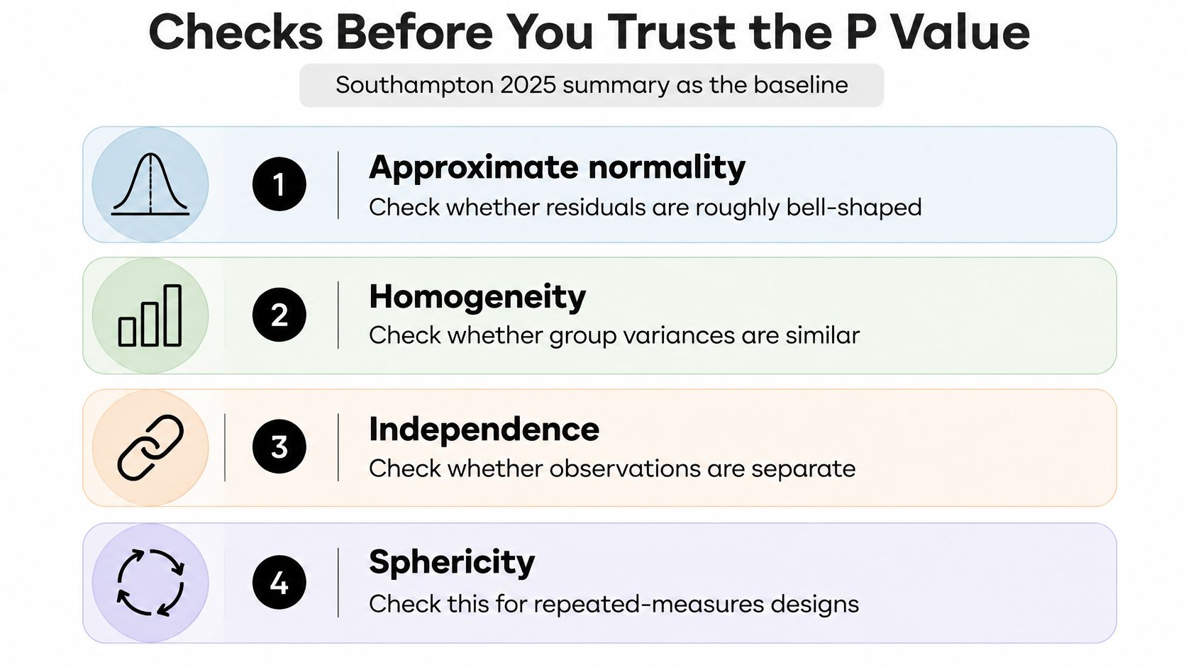
The checklist summarizes the standard diagnostic categories; the working sequence should still begin with independence.
Inspect residual shape and group spread
Approximate normality concerns model errors, assessed through residuals, not the pooled outcome distribution. Pooling groups with different means can produce an unusual-looking distribution even when within-group residuals behave reasonably.
Inspect a residual Q-Q plot, residuals against fitted values, and the observations within each group. Mild departures may be tolerable, especially with balanced samples, but severe skew, heavy tails, or influential outliers deserve investigation. A Shapiro-Wilk test can flag small, unimportant departures in a large sample, so don't use its p-value as an automatic stop signal.
For a regression-oriented diagnostic reference, Model Diplomat's tools for checking regression analysis are relevant because classical ANOVA is also a linear-model analysis. Use diagnostic tools to inspect the fitted model, not to replace judgment about the sampling design.
Homogeneity of variance means residual spreads are reasonably similar across groups. Examine group plots and consider Levene's or Brown-Forsythe testing, while remembering that a non-significant test doesn't prove equal variance. Our explanation of homoscedasticity connects this assumption to residual patterns.
Match the remedy to the problem
Different failures call for different changes:
- Unequal independent-group variances: Consider Welch ANOVA rather than the classical pooled-variance F-test.
- Strong skew or unsuitable outcome distribution: Consider a scientifically interpretable transformation or a generalized linear model with a suitable likelihood.
- Clustering or repeated observations: Include the dependence structure explicitly.
- Unusual observations: Check recording errors and influence before deciding whether any exclusion is defensible.
For repeated measures, sphericity concerns the variances of differences between pairs of conditions or times. Mauchly's test evaluates that restriction; Greenhouse-Geisser or Huynh-Feldt corrections adjust the inferential degrees of freedom when appropriate. They don't restore missing visits or turn an unsuitable longitudinal design into a complete one.
A failed diagnostic is a reason to reconsider a specific modeling assumption, not permission to select whichever test produces the preferred p-value.
Sample size also affects interpretation. Sparse cells make interactions imprecise, while enormous samples can make negligible differences look decisive. Report uncertainty and assess practical importance rather than treating the p-value as a complete conclusion.
Don't jump to ranks by reflex. Changing from a mean-based analysis to a rank-based analysis changes what you're testing.
One-Way Two-Way and Repeated Measures
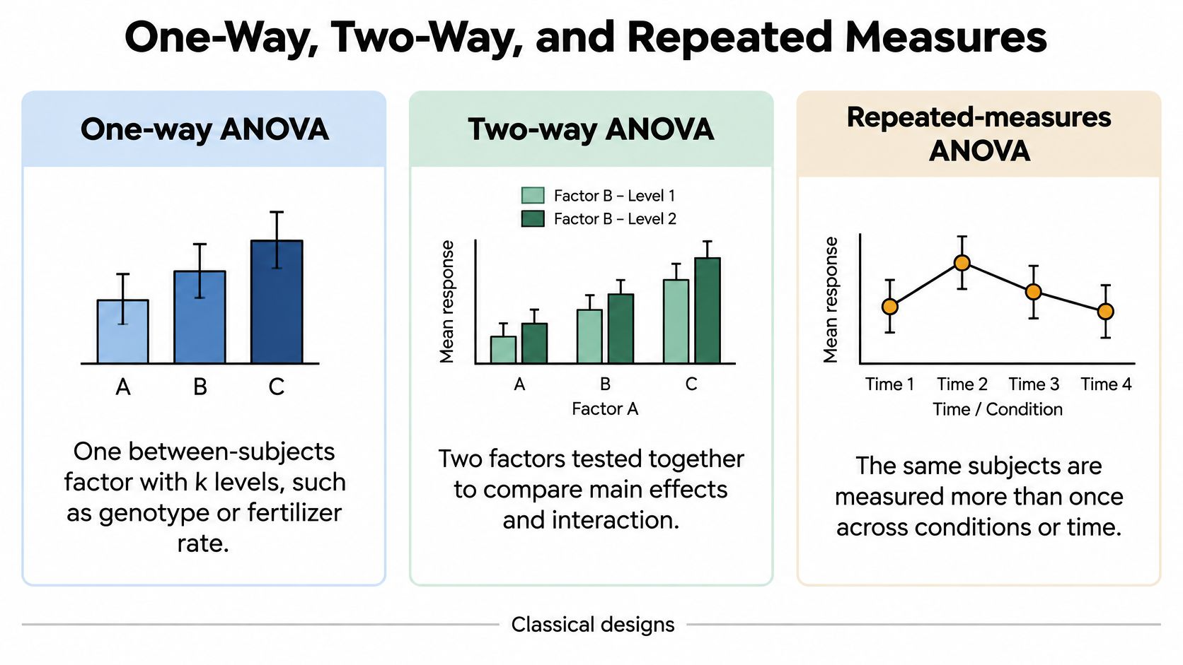
The word way refers to the factors in the design, not the number of groups or spreadsheet columns. The distinction matters because adding a factor can change both the scientific question and the meaning of the estimated effects.
These classical designs organize different kinds of comparisons.
One-way designs compare levels of one factor
Suppose an agricultural researcher assigns genotypes to independently randomized experimental units. Genotype is the factor, and each genotype is a level. One-way ANOVA asks whether the population mean outcome is equal across those levels.
The experimental unit deserves particular attention. Measuring several leaves from the same plant doesn't necessarily create independent treatment replicates. If treatment was assigned to the plant, leaf measurements are subsamples, and the analysis must preserve that hierarchy.
A clean one-way model is useful when the grouping factor captures the comparison of interest and no omitted design structure requires modeling. A blocked field experiment isn't made one-way merely by leaving the block column out.
Two-way designs estimate interactions
Now cross genotype with irrigation regime. A two-way model estimates genotype and irrigation main effects plus their interaction.
An interaction means the effect of one factor changes across levels of the other. A genotype might outperform another under adequate irrigation but not under drought. Reporting only an average genotype effect could conceal the finding that matters for deployment.
Balanced cells simplify classical interpretation because factor effects are more cleanly separated. With unbalanced observational groups, specify which means and weighting scheme you intend to compare. Different sums-of-squares choices can correspond to different hypotheses, so the software default isn't a scientific justification.
Adding continuous covariates moves the analysis toward ANCOVA, or a more general linear model. Covariate adjustment can address measured differences, but it doesn't remove clustering or guarantee control of confounding.
Repeated measures need a deliberate mixed-model decision
Repeated-measures ANOVA is most defensible when each participant is observed at every level of a simple within-subject factor, the measurement grid is complete, and its covariance assumptions are appropriate. A participant measured under each laboratory condition is a straightforward example.
A methodological review of repeated-measures analysis explains why mixed-effects models offer greater flexibility for incomplete or unbalanced longitudinal data and covariance structures that don't satisfy strict sphericity.
Use this explicit switch rule:
- Prefer repeated-measures ANOVA: Complete, balanced observations and a simple within-subject comparison.
- Consider a mixed model: Missing visits, uneven measurement times, participant-specific baselines or slopes, or correlations that change with time separation.
Clinical visits, classroom assessments, and policy panels often create the latter situation. Nearby observations may be more correlated than distant observations, and participants may begin at different levels or change at different rates.
A mixed model still requires defensible assumptions. Its ability to retain incomplete records doesn't make informative dropout harmless; investigate why observations are missing and consider sensitivity analyses.
Our guide to repeated-measures ANOVA develops the within-subject setup in more detail.
Tie the choice to the estimand. An omnibus time-by-group test asks whether mean profiles differ somewhere. A suitably specified mixed model can instead estimate average change per week, treatment differences at a target visit, or variation in subject-specific trajectories.
Contrasts Post-Hoc Tests and Other Models
Before selecting a follow-up procedure, ask which comparisons belong to the scientific question. A treatment-versus-standard comparison and an exploratory search across every pair aren't interchangeable tasks. They need different multiplicity plans.
A planned contrast can compare particular means or a weighted combination of means. For example, a researcher might compare standard care against the average of several active treatments. That hypothesis isn't necessarily best represented by testing every possible pair.
Planned hypotheses and exploratory comparisons
A 2025 methodological preprint on comparison procedures argues for Bonferroni adjustment when researchers have a limited set of pre-specified comparisons rather than automatically conducting all-pairs Tukey testing. That's one defensible methodological position, not settled consensus that Tukey should generally be abandoned.
Tukey HSD remains a standard all-pairs procedure when every pair is of interest and its model assumptions are appropriate. Similar group sizes make the basic setting straightforward; Tukey-Kramer handles unequal sample sizes under the equal-variance model. Games-Howell is a common alternative for pairwise comparisons with unequal variances.
Planned contrasts don't require a significant omnibus F-test first. Whether an omnibus test acts as a gate should follow the pre-specified testing strategy, not a habit adopted after seeing results.
Follow-up comparison or a different model
| Situation | Report this | Do not default to |
|---|---|---|
| A few contrasts specified in advance | Contrast, confidence interval, Bonferroni or other preset adjustment, number of tests | All-pairs Tukey |
| All pairs of interest after a valid ANOVA | Tukey HSD intervals under similar variance and sample size | Unadjusted t-tests on every pair |
| Independent groups with unequal spreads | Welch ANOVA and Games-Howell if pairs are needed | Classical F then Tukey |
| Ordinal, binary, or count outcome | Ordinal model or GLM with the right likelihood | ANOVA on the raw codes |
| Rank-based omnibus interest only | Kruskal-Wallis, described as a rank test | Calling Kruskal-Wallis a test of means |
For each comparison, report the contrast estimate, confidence interval, multiplicity method, and number of comparisons. State whether the interval itself is multiplicity-adjusted. Our multiple-testing correction guide explains how the comparison family affects that decision.
Effect sizes should match the design and question. Omega-squared estimates an omnibus share of variance associated with the factor; partial eta-squared is common for terms in factorial models. Neither replaces the mean difference in clinically or scientifically meaningful units.
Avoid interpreting partial eta-squared as a universally comparable proportion of all outcome variation. Its denominator is conditional on the model term and associated error, so comparisons across designs require care.
For binary outcomes, consider logistic regression; for counts, choose a suitable count model; for ordered categories, consider an ordinal model. A numeric label doesn't justify averaging categories whose spacing has no substantive meaning.
Kruskal-Wallis tests differences in rank distributions. Under additional shape assumptions it can support a location interpretation, but it isn't an automatic test of medians and isn't a test of means. Choose it because the rank-based question fits, not because a normality test was significant.
Three Examples and How to Read Them
The following are constructed teaching examples, not published trials. Their numbers illustrate how design, uncertainty, and the reporting sentence fit together. They don't establish real fertilizer or analgesic effects.
The visual distinguishes common comparison structures; the worked examples below focus on one-way, factorial, and longitudinal analyses.
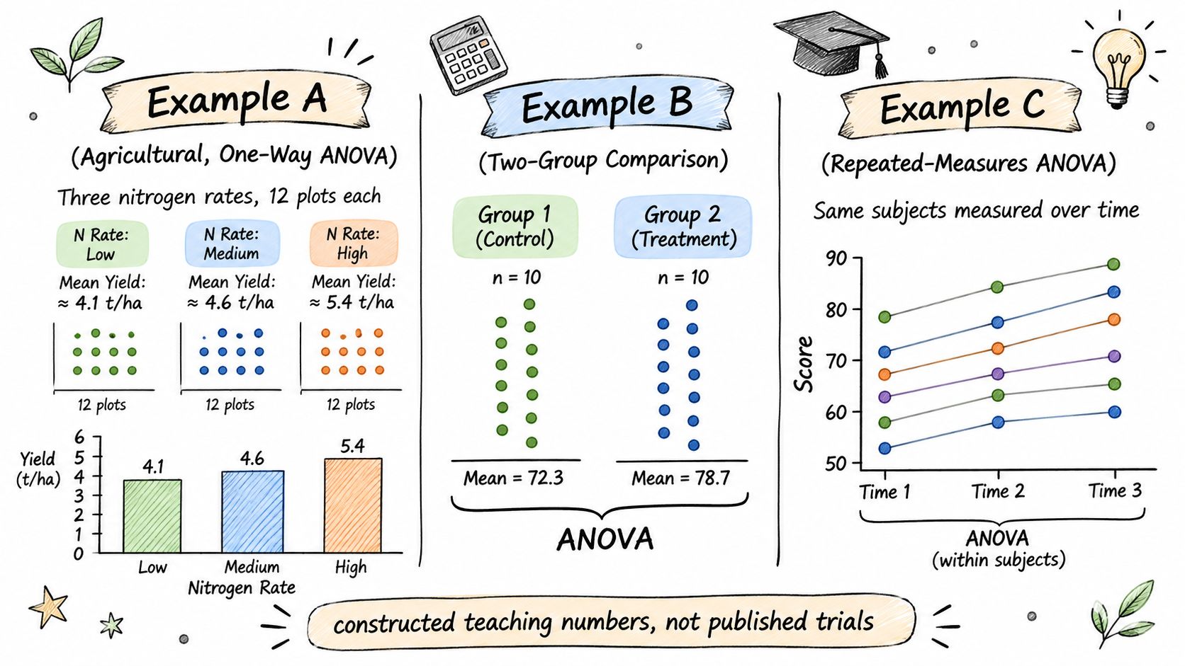
Example A compares nitrogen rates
Suppose three nitrogen rates are independently randomized to 12 plots each. Constructed group means are 4.1, 4.6, and 5.4 tonnes per hectare, with a pooled residual standard deviation of 0.8 tonnes per hectare.
These summary values give F(2, 33) ≈ 8.06, with p < 0.01, and omega-squared ≈ 0.28. The effect-size estimate suggests a substantial share of yield variation associated with rate in this hypothetical design, but its precision still depends on the sample.
At a conventional illustrative 95% family-wise confidence level, Tukey intervals for medium minus low, high minus low, and high minus medium are approximately −0.30 to 1.30, 0.50 to 2.10, and 0.00 to 1.60 tonnes per hectare, respectively. The last lower endpoint is slightly below zero before rounding, so it shouldn't be described as clearly excluding zero.
The honest sentence is that mean yields differ across rates, with clear evidence for high versus low, not that every observed rank is confirmed. Report all intervals and the effect-size definition, and don't turn an unresolved comparison into a claim of equality.
Worked example results (illustrative teaching numbers)
| Example | Design | Key numbers | Reporting action |
|---|---|---|---|
| A, one-way nitrogen rates | Three independent rates, 12 plots per rate | Means 4.1, 4.6, 5.4 tonnes/hectare; residual SD 0.8; F(2, 33) ≈ 8.06; p < 0.01; omega-squared ≈ 0.28 | Report means with intervals, omnibus result, effect size, and exact rate contrasts |
| A, Tukey follow-up | All three pairs | Low vs medium interval includes zero; low vs high interval excludes zero | Report the three intervals, not one omnibus p-value |
| B, two-way analgesic | Dose by sex, 20 people per cell | Constructed interaction p ≈ 0.02; high dose helps more in one sex | Plot the four cell means before any pooled dose claim |
| C, repeated pain scores | 30 patients at baseline, week 2, week 4 | Complete data: repeated-measures ANOVA if sphericity holds | 8 missing week 4: refit as a mixed model for average change |
Example B centers the interaction
Consider a constructed pain-reduction study crossing low versus high analgesic dose with sex, with 20 participants per cell. Suppose the fitted interaction has p ≈ 0.02, and the high dose produces a greater improvement in one sex.
Plot the four cell means with intervals. Then estimate the dose difference within each sex and the difference between those dose differences, which directly expresses the interaction.
The p-value alone doesn't supply those magnitudes or permit calculation of a unique partial eta-squared without the test details. A complete report needs cell means, intervals, interaction degrees of freedom, the chosen effect size, and the planned simple-effect contrasts. Cell size also limits how precisely the interaction can be estimated.
For a simpler independent or paired comparison without a factorial question, the sample t-test guide provides the corresponding setup.
The following video offers an additional explanation of ANOVA.
Example C changes when visits are missing
Suppose 30 patients provide pain scores at baseline, week 2, and week 4. With complete data and suitable difference-score variances, repeated-measures ANOVA on time is reasonable.
If 8 patients miss week 4, don't automatically delete those patients and repeat the original analysis. Reconsider the target population and missingness mechanism, then fit a mixed model aimed at average change if its assumptions are defensible.
Report visit means with intervals, the exact target contrast, such as week 4 minus baseline, and an effect measure suited to that model. A single-group time trend doesn't establish a treatment effect because other changes over time remain possible.
Across these examples, inspect influential observations and variance patterns. Refit using a justified sensitivity analysis and state whether the substantive conclusion changes. Keep plots used to discover a pattern distinct from contrasts specified before inspecting outcomes.
Choose the Test Then Investigate the Data
Before opening software, write the comparison in a sentence. For example: “Estimate the average difference in pain scores between week 4 and baseline among patients with observed outcomes.” That sentence identifies what the analysis should estimate. The model must then match the outcome, study design, and observations available.
Use four steps:
- Specify the target. Name the outcome, factors or time structure, independent sampling unit, and planned contrast.
- Check relevant assumptions. Inspect residuals and group spreads. For repeated measures, examine covariance and missingness as well.
- Report estimates and uncertainty. Include group or cell means, an effect size suited to the design, and planned contrasts with the multiplicity method and number of comparisons.
- State the limits. Separate association from causation, uncertainty from evidence of equivalence, and a defensible model from a software default.
Where agentic analytics helps
Agentic analytics uses AI agents to plan an investigation, run analysis with tools and code, inspect results, revise steps when needed, and present findings. A chatbot answer may give a conclusion; an analysis should also show how that conclusion was reached.
PlotStudio AI can profile an uploaded dataset and, given a clear research question, propose an analysis plan, execute Python locally, and save the code, charts, tests, and interpretation on a permanent Analysis Page. Verification Mode lets researchers review and edit the plan before analysis runs, inspect a summary of changes, and undo edits. The resulting page keeps the findings together for review.
Automation can make the work easier to inspect and reproduce. It cannot decide which estimand matters or make unsupported missingness assumptions valid. Researchers still need to justify the comparison and interpret the result in context.
Frequently asked questions
When should I use ANOVA instead of a t-test?
Use ANOVA to compare means across multiple factor levels or to assess a factorial design. For one independent or paired comparison, a matching t-test is usually clearer.
Does significant ANOVA mean every group differs?
No. The F test indicates evidence against the overall null hypothesis, not that every pair differs. Report the contrasts that answer the research question, with estimates and adjusted uncertainty.
Can I use ANOVA with missing repeated measurements?
A mixed model may be more suitable than excluding everyone with an incomplete set of measurements. Investigate the missingness and justify the model assumptions.
Should I always run Tukey after ANOVA?
No. Tukey is designed for all-pairs comparisons. If the research question specifies particular contrasts, report those instead, using an appropriate method to account for multiple comparisons.