Quantile regression models a chosen conditional quantile of an outcome, such as the median or the 90th percentile, rather than its mean, by minimizing pinball loss. If a predictor changes the upper tail more than the middle, why summarize its association with a single average slope?
What Quantile Regression Models
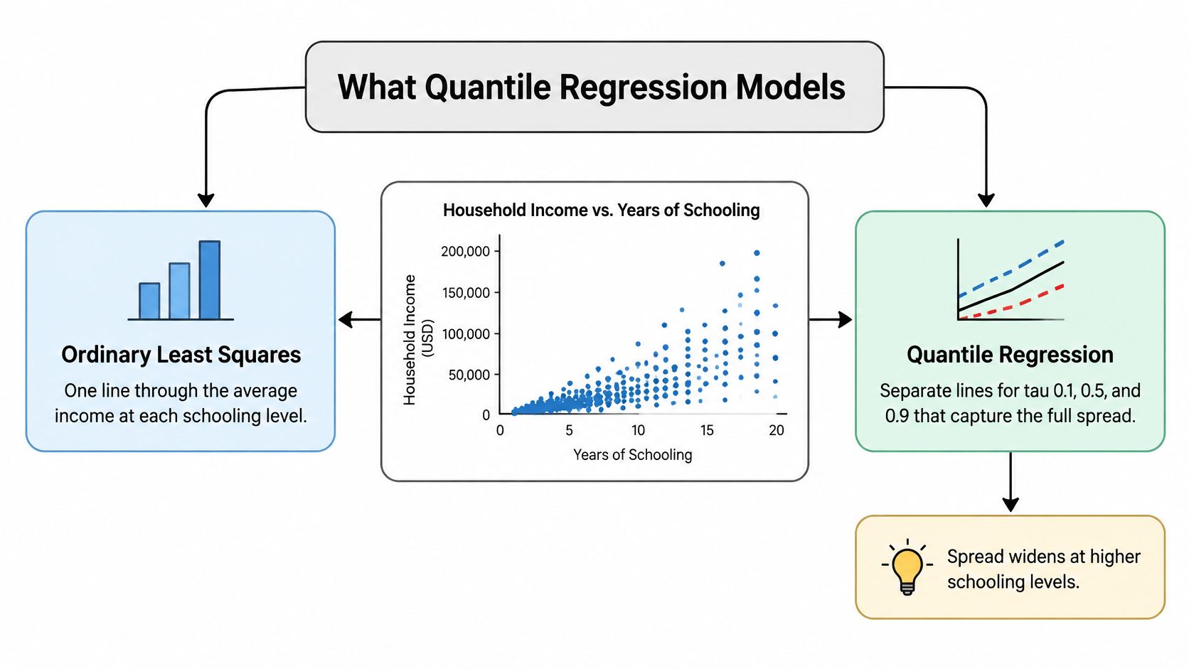
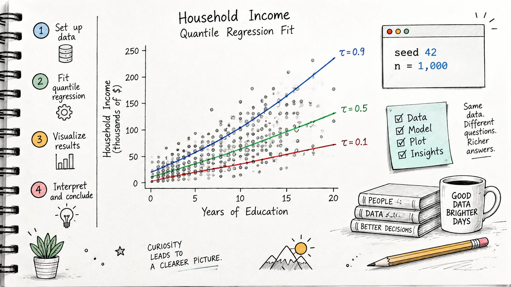
Consider a hypothetical scatter plot of household income against years of schooling. At lower schooling levels, incomes cluster relatively tightly; at higher levels, they spread farther apart. An ordinary least squares line summarizes average income at each schooling level, but it doesn't describe how the lower and upper parts of that conditional distribution differ.
Think of a crowd photographed from the side. OLS places a ruler through its center; quantile regression places separate rulers along lower, middle, and upper positions. Those rulers can tilt differently. They're summaries of positions in a distribution, not labels attached permanently to particular people.
From the picture to the model
The foundational Koenker and Bassett formulation defines regression quantiles through a quantile level (\tau \in (0,1)) and the linear specification:
[
Q_Y(\tau \mid X)=X^T\beta(\tau).
]
Here, (Q_Y) is the chosen conditional quantile, and (X) contains the predictors, including an intercept. The important addition is (\beta(\tau)): the coefficient vector carries a quantile label because each chosen quantile can have its own slopes.
For example, (\tau=0.5) targets the conditional median, while (\tau=0.9) targets the conditional upper percentile. A slope describes the change in that modeled quantile associated with a unit increase in a predictor, holding the other included predictors fixed.
Reading a hypothetical schooling slope
Suppose a model of log household income returns schooling slopes of 0.03 at the lower quartile and 0.09 at the upper decile. These are illustrative coefficients, not empirical findings. They would indicate a larger schooling association with the upper conditional quantile on the log-income scale.
- The predictor is years of schooling.
- The target is a specified conditional quantile of log income.
- The comparison holds the other included covariates fixed.
The coefficient path across quantiles answers the useful question: where in the conditional outcome distribution does the predictor have a larger association?
The Pinball Loss Behind the Estimator
Take a hypothetical household with income recorded as 60 units. At (\tau=0.9), predicting 50 creates a positive residual of 10 and a loss of 9; predicting 70 creates a negative residual of −10 and a loss of 1. Equal-sized mistakes receive unequal penalties because the target is an upper quantile.
The loss diagram shows that asymmetry.
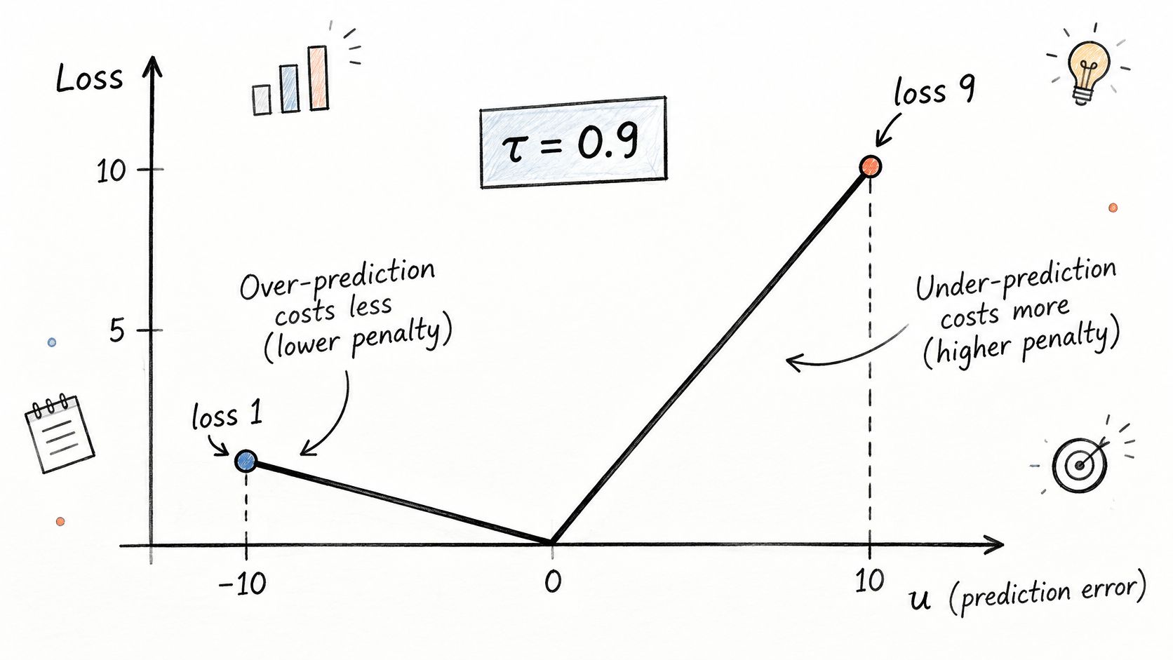
With residual (u) defined as observed outcome minus fitted value, the pinball loss, also called check loss, is:
[
\rho_\tau(u)=u[\tau-I(u<0)].
]
The indicator (I(u<0)) identifies overprediction. Underprediction receives weight (\tau), while overprediction receives weight (1-\tau). Think of a weighing scale that charges more for missing in one direction than the other.
Penalty weights and targets for common quantile levels
| Quantile level tau | Weight on underprediction | Weight on overprediction | What the fit targets |
|---|---|---|---|
| 0.25 | 0.25 | 0.75 | First quartile |
| 0.50 | 0.50 | 0.50 | Median, least absolute deviations |
| 0.75 | 0.75 | 0.25 | Third quartile |
These weights follow directly from the loss definition. At the median, the objective is proportional to absolute deviation, so multiplying the entire objective by a constant doesn't change the minimizing coefficients.
In an intercept-only model, minimizing summed pinball loss returns a sample quantile. Adding predictors generalizes that idea: instead of estimating a single distributional cutoff, the analyst estimates how the cutoff changes with covariates.
Why numerical optimization is needed
The objective is piecewise linear and has a corner at a zero residual. General quantile regression therefore doesn't have the familiar OLS matrix solution; implementations use linear programming, including simplex or interior-point approaches, or iterative methods such as iteratively reweighted least squares.
The accompanying video provides another visual explanation of the objective.
Practical rule: The fitted line approximates a conditional quantile under the chosen specification. It doesn't guarantee the requested fraction below the line within every possible subgroup.
That distinction matters when a straight line poorly represents the relationship or when some covariate combinations have little support.
How Quantile Regression Differs From OLS
| Aspect | OLS | Quantile regression |
|---|---|---|
| Target | Conditional mean (E[Y\mid X]) | Conditional quantile (Q_Y(\tau\mid X)) |
| Loss function | Squared error | Pinball loss with asymmetric weights |
| Slopes returned | One slope per predictor | One slope per predictor per quantile |
| Outliers in the outcome | Can pull the fitted line toward them | Residual contribution to the score is bounded by its side |
| High-leverage predictor values | Influential | Still influential; check predictor-space extremes |
| Heteroskedasticity | Models the mean despite changing spread | Quantile paths can reveal changing spread or shape |
| Error assumptions for inference | Exact classical small-sample inference uses normal errors | No normality requirement; density near the quantile matters |
| Computation | ((X^TX)^{-1}X^Ty), when full rank | Linear programming or IRLS; no general closed form |
Choose the estimand before choosing the estimator. If the scientific question concerns average blood pressure, an OLS mean model may be appropriate even when the outcome distribution is asymmetric. Heteroskedasticity doesn't automatically invalidate the mean coefficient estimates, although conventional homoskedastic standard errors can be inappropriate.
The predictor structure remains familiar. You can include adjustment covariates, interactions, and nonlinear terms, just as in multiple regression.
When the fitted slopes agree
Under a correctly specified location-shift model with errors independent of the predictors and a constant distributional shape, quantile lines have common slopes and different intercepts. With symmetric, centered errors, mean and median regression describe the same central relationship, although sample estimates needn't match exactly.
Symmetry alone isn't enough to make every quantile slope equal. If the error scale changes with a predictor, upper and lower quantile slopes can separate even when the conditional distribution remains symmetric.
What robustness does and doesn't mean
An extreme outcome can move the OLS line substantially because squared loss increasingly penalizes large residuals. In quantile regression, loss still grows with residual magnitude, but its derivative with respect to the residual depends on the residual's side rather than increasing with its size.
That provides response-side resilience, not immunity to problematic observations. A household with an extreme schooling value can still exert substantial influence.
Use OLS when the mean is the question. Add quantile regression when the scientific question concerns distributional position, unequal spread, or tail behavior.
Neither method automatically resolves confounding, measurement error, or an incorrectly specified predictor relationship.
Estimation and Bootstrap Inference
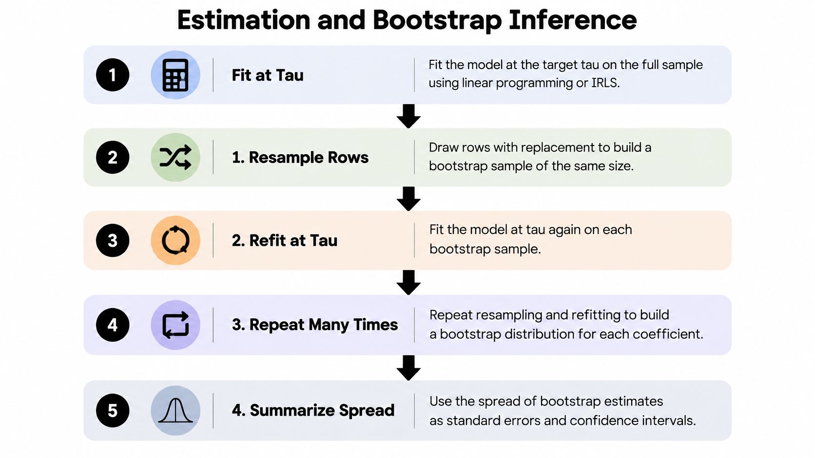
Fit the target quantile on the full analysis sample before estimating uncertainty. The statsmodels QuantReg implementation uses iteratively reweighted least squares and supports sandwich or iid covariance estimates, kernel choices, bandwidth settings, and convergence controls.
For independent observations, a pairs bootstrap provides a practical alternative uncertainty calculation:
- Fit the model at the chosen (\tau) on the full sample.
- Draw (n) rows with replacement, keeping each outcome and its predictors together.
- Refit the same specification at the same quantile.
- Store the resulting coefficient vector and any convergence warnings.
- Repeat for a prespecified number of replicates. For a worked analysis, start with 500, then increase toward 1,000 or more and assess interval stability, especially in the tails.
- For a 95% percentile interval, take the 2.5th and 97.5th percentiles of the bootstrap coefficient estimates.
These replicate counts are workflow choices, not guarantees of reliable coverage.
Why the resampling unit matters
Pairs resampling retains each observed predictor-outcome pairing, preserving the empirical relationship between covariates and changing outcome spread. It doesn't force residuals from different predictor settings to share a common distribution.
Rows aren't the right unit when observations are dependent. For students nested in schools or repeated measurements within patients, resample whole independent clusters, retaining their observations together. Ignoring that dependence can understate uncertainty.
Kernel inference versus bootstrap inference
Asymptotic quantile-regression standard errors depend on the conditional error density near the target quantile. Kernel estimation therefore introduces bandwidth and kernel choices; sandwich covariance estimation is preferable when error scale changes with covariates.
A pairs percentile bootstrap avoids an explicit density-bandwidth choice for interval construction, but every replicate requires another model fit. It also requires adequate independent sampling units and regularity conditions. It isn't automatically more reliable in sparse tails.
For interpretation, distinguish an interval for a coefficient from an interval describing outcome variability. The guide to understanding confidence intervals explains the uncertainty distinction.
Wide or asymmetric tail intervals often reflect limited information, but they can also reveal instability or misspecification. Check the data support and solver output before treating them as routine.
Python Example With Statsmodels and a Quantile Plot
Use a simulation with known answers before analyzing a clinical or socioeconomic dataset. The following is a constructed heteroskedastic model, not an empirical result: (y=1+2x+(0.5+0.5x)\varepsilon), with standard normal (\varepsilon) independent of (x).
Generate data and fit the models
First, initialize the random generator and simulate the sample. Then fit the quantile grid and an OLS baseline.
import numpy as np
import pandas as pd
import statsmodels
import statsmodels.formula.api as smf
import matplotlib.pyplot as plt

rng = np.random.default_rng(42)
n = 1000
x = rng.uniform(0, 10, n)
y = 1 + 2*x + (0.5 + 0.5*x)*rng.standard_normal(n)
df = pd.DataFrame({"x": x, "y": y})
taus = np.array([0.10, 0.25, 0.50, 0.75, 0.90])
fits = {
t: smf.quantreg("y ~ x", df).fit(
q=t, vcov="iid", max_iter=10000
)
for t in taus
}
ols = smf.ols("y ~ x", df).fit()
rows = []
for t, fit in fits.items():
    low, high = fit.conf_int().loc["x"]
    rows.append((t, fit.params["x"], low, high))
results = pd.DataFrame(
    rows, columns=["tau", "slope", "low", "high"]
)
print(results)
print("statsmodels version:", statsmodels.__version__)
The expected pattern is a larger slope at higher quantiles. For this constructed model, the true slope is (2+0.5z_\tau), where (z_\tau) is a standard normal quantile, giving approximately 1.36 and 2.64 at the lower and upper fitted deciles.
True slopes for the simulated model
| Quantile tau | Standard normal quantile | True slope 2 + 0.5 z |
|---|---|---|
| 0.25 | −0.67449 | 1.66276 |
| 0.50 | 0 | 2 |
| 0.75 | 0.67449 | 2.33724 |
These are calculated benchmarks, not fitted output. Sampling variation means the estimates won't equal them exactly.
Next, plot both the fitted outcome lines and the coefficient path.
grid = pd.DataFrame({"x": np.linspace(x.min(), x.max(), 200)})
fig, axes = plt.subplots(1, 2, figsize=(12, 4))

axes[0].scatter(x, y, s=8, alpha=0.2)
for t, fit in fits.items():
    axes[0].plot(grid.x, fit.predict(grid), label=f"tau={t:.2f}")
axes[0].plot(grid.x, ols.predict(grid), "k:", label="OLS")
axes[0].set(xlabel="x", ylabel="y")
axes[0].legend()

axes[1].plot(results.tau, results.slope, marker="o")
axes[1].fill_between(
    results.tau.to_numpy(),
    results.low.to_numpy(),
    results.high.to_numpy(),
    alpha=0.2
)
axes[1].axhline(ols.params["x"], color="black", linestyle=":")
axes[1].set(xlabel="Quantile tau", ylabel="x coefficient")
plt.tight_layout()
plt.show()
The first panel should fan outward; the second should show an increasing coefficient path. Its shaded intervals are pointwise, not a simultaneous confidence band.
Compare the upper-quantile interval with a bootstrap
Finally, refit the upper quantile on resampled rows.
boot_slopes = []
for _ in range(500):
    sample = df.iloc[rng.integers(0, n, size=n)]
    fit = smf.quantreg("y ~ x", sample).fit(
        q=0.90, max_iter=10000
    )
    boot_slopes.append(fit.params["x"])

print("Bootstrap:", np.quantile(boot_slopes, [0.025, 0.975]))
print("Kernel-based:", fits[0.90].conf_int().loc["x"].to_numpy())
Inspect warnings rather than silently suppressing them. Save the script, seed, data-generation specification, and package versions; pin the installed statsmodels version in your environment file. For environment management and reusable scripts, use the Python for statistical analysis guide.
Diagnosing Quantile Fits and Fixing Them
Start with inexpensive checks: inspect convergence warnings, plot the fitted quantiles, and compare the coefficient path with the OLS baseline. A successful function call doesn't establish that the model is scientifically appropriate.
Quantile regression symptoms, causes and fixes
| Symptom | Likely cause | Fix |
|---|---|---|
| Quantile lines cross over part of the x range | Separate fits without a monotonicity constraint | Locate the crossing region; restrict presentation or apply rearrangement and report it |
| Slopes nearly identical across tau | A location-shift pattern or insufficient evidence of heterogeneity | Test slope equality; a simpler location model may be adequate |
| Very wide intervals at tau = 0.05 or 0.95 | Few informative observations near the tail | Collect more data, narrow the quantile grid, and report uncertainty |
| Solver stops without converging | Collinearity, poor scaling, or excessive complexity | Scale predictors, remove redundant terms, and consider increasing max_iter |
| Bootstrap intervals change between runs | Monte Carlo instability; possibly inappropriate resampling | Increase replicates and use cluster resampling when the design requires it |
| Predicted quantiles outside the observed range | Potential extrapolation or model mismatch | Check predictor support; restrict unsupported predictions |
Predictions outside observed outcome values aren't automatically invalid. The important question is whether the model extrapolates beyond supported predictor combinations or violates a known outcome boundary.
Check ordering and coefficient differences
Evaluate every fitted quantile at a common grid of predictor values. With several predictors, inspect scientifically relevant covariate profiles and observed combinations, not just a line through their averages.
For the simulation, an ordering check is straightforward:
predictions = np.column_stack([
    fits[t].predict(grid).to_numpy() for t in taus
])
crossing = np.any(np.diff(predictions, axis=1) < 0, axis=1)
print("Crossing detected:", crossing.any())
To compare slopes, refit all relevant quantiles within the same bootstrap resample, then calculate their difference. This retains the dependence between coefficient estimates. Comparing whether separately reported confidence intervals overlap isn't a valid substitute for directly estimating the difference.
Diagnostic caution: Rearrangement restores numerical ordering. It doesn't explain why the original specifications crossed.
Report where crossing occurred and whether the affected covariate region had adequate observations. A constrained model, nonlinear terms, or narrower prediction scope may be more defensible than cosmetic repair.
Use a broader regression diagnostics workflow to examine influence, specification, and data quality. Near-identical slopes alone don't establish that the conditional mean model is correct.
Interpreting Coefficients Without Overstating Scope
A 90th-percentile coefficient does not generally describe the top 10% of people. It describes a conditional distributional position at specified covariate values, not a fixed set of individuals.
Suppose a wage model includes schooling, experience, and region. The schooling coefficient at an upper conditional quantile compares that wage quantile across schooling values while holding experience and region fixed. It doesn't identify what would happen to a permanent group of high earners if their schooling changed.
Conditional and population questions aren't interchangeable
The distinction between conditional quantile regression, unconditional quantile regression, and quantile treatment effects is examined in this sociological methods study. Conditional and unconditional quantiles don't aggregate linearly, so a conditional lower-quartile association generally isn't the change in the overall population's lower quartile.
Unconditional quantile methods, often using recentered influence functions, address population-distribution questions under their own specifications and assumptions. Quantile treatment effects concern contrasts between potential-outcome distributions; they aren't interchangeable with either conditional regression coefficients or unconditional regression coefficients.
None of these labels establishes causality. An observational schooling coefficient may reflect confounding, selection, measurement error, or omitted variables. Adjustment makes the comparison conditional on included covariates, not necessarily causally identified.
A reporting checklist
- Name the quantile. Identify the target rather than saying only “tail effect.”
- State the estimand. Specify conditional association, unconditional distributional change, or a justified causal contrast.
- List the adjustment variables. Explain what the comparison holds fixed.
- Give the outcome scale. Dollars and log wages require different interpretations.
- Report uncertainty. Include coefficient intervals and uncertainty for planned cross-quantile contrasts.
- Define the population. Describe sampling, exclusions, and the population to which conclusions apply.
A guide to interpreting regression results can help keep coefficient language aligned with the model.
Prespecify scientifically meaningful contrasts when possible. If you explore many predictors and quantiles, distinguish exploratory patterns from confirmatory conclusions and address multiplicity rather than selecting only the most striking coefficient.
Frequently Asked Questions
Is quantile regression the same as median regression?
Median regression is a special case. Selecting the middle quantile gives equal penalties on either side of a residual and produces the least absolute deviations fit. Other quantile levels answer different distributional questions.
Which software fits quantile regression?
Python's statsmodels provides QuantReg and the formula interface smf.quantreg. R offers Koenker's quantreg package, while Stata provides qreg and bsqreg.
Choose software that supports the inference your sampling design requires and lets you preserve executable code, diagnostics, and model settings.
Can an AI tool run quantile regression for me?
An AI tool can generate and execute Python, inspect convergence, and produce plots. The researcher still defines the estimand, chooses adjustment variables, assesses the sampling design, and decides whether the interpretation is justified.
Ask for inspectable code and diagnostic output, not just a polished explanation.
Should I remove missing observations before fitting?
Establish the missing-data strategy before fitting. Record which variables cause exclusions and whether the analysis sample changes across specifications.
Complete-case analysis isn't automatically appropriate. If you use imputation, ensure the imputation strategy and uncertainty calculation are compatible with the scientific question and analysis model.
Set the Question and Quantile Grid Before Fitting
Which part of the outcome distribution should your analysis explain? Choose quantiles to answer that scientific question, rather than to produce appealing results. A practical starting grid is 0.10, 0.25, 0.50, 0.75, and 0.90. Consider 0.05 and 0.95 only if the sample and design support credible tail estimates.
Treat each quantile as its own question. Before fitting, write down the estimand, fix the quantile grid, and specify any planned contrasts. Then fit an OLS baseline and the quantile models on a documented analysis sample. Check convergence, predictor support, and whether fitted quantiles cross. Estimate uncertainty with intervals suited to the design, using bootstrap intervals where useful. Save code, settings, diagnostics, and outputs so another analyst can reproduce the investigation.
Agentic analytics is data analysis performed by AI agents that plan an investigation, execute steps with tools and code, inspect intermediate results, revise the approach, validate outputs, and synthesize an analysis. An answer is an output; an analysis is an investigation.
PlotStudio AI helps researchers investigate data rather than merely chat about it. It can run a planned local Python analysis and preserve code, plots, and methodology in a reproducible Analysis Page. Its cleaner documents transformations, including dropped row counts, imputations, and recodings, making data preparation auditable. The researcher remains responsible for statistical decisions, including which quantiles to fit and how to interpret their coefficients. Those coefficients describe conditional quantiles, not automatically population subgroups or individual outcomes. Comparing coefficient paths across quantiles shows where a predictor's association differs across the conditional outcome distribution.