The 1 sample t test formula is t = (x̄ − μ₀) / (s / √n). You subtract the hypothesized mean from your sample mean, divide by the standard error of the mean, and compare the result to a critical value from the t distribution with n − 1 degrees of freedom. A large t means your sample mean sits far from the hypothesized value, relative to how much sample means normally vary.
In plain terms, the one-sample t-test asks whether the average of one group differs from a number you already have. That number might be a reference value, a label claim, or a regulatory limit. The test is built for the usual situation where the sample is small to moderate and the population standard deviation is unknown.
This article explains why the formula is worth learning and what every symbol does. It then walks one dataset through the calculation by hand, shows how to read the result, and lists the mistakes that most often break it. At PlotStudio AI we build tools that run these tests on research data, and we still recommend learning the hand calculation first. You should be able to verify any output you report.
Why the one-sample t-test formula matters
You need this formula because it answers the most common single-group question in research: is my sample mean different from a number I already know? Every other t-test is a variation on the same ratio, so learning it once makes the rest easier.
What the test answers
The test compares one sample mean to a fixed reference value, called the hypothesized or test value. That value comes from theory, a published standard, a label claim, or an earlier study. You might compare mean hemoglobin in a patient group to a clinical reference, or check whether a production line fills containers to the labeled volume.

The test also handles change scores. Subtract the before measurement from the after measurement for each participant, then test whether the mean difference equals zero. That is a paired t-test, and underneath it is the one-sample formula with μ₀ = 0.
A one-sample t-test asks whether your sample mean sits too far from a reference value to blame chance.
One sample, two samples, or paired
Choose the test by looking at how your data are organized, not at the topic of your study.
| Your design | Test to use | Hypothesized value |
|---|---|---|
| One group compared with a known value | One-sample t-test | A fixed number, μ₀ |
| Same participants measured twice | Paired t-test (one-sample on the differences) | 0 |
| Two separate groups | Independent two-sample t-test | Usually a difference of 0 |
If you have a single column of numbers and one value to compare it to, use the one-sample test. If you have two columns from two different groups, you need a different formula.
Assumptions to check first
The formula returns a number whatever your data look like, so check these conditions before you trust it:
- The outcome is continuous, such as a measurement rather than a category.
- Observations are independent. One value does not influence another.
- The sample is random, or at least representative of the population you care about.
- The population is approximately normal, or the sample is large enough that the mean behaves normally.
Normality matters most in small samples. With moderate or large samples, mild skew does little harm. With a small sample that has heavy skew or clear outliers, a nonparametric alternative such as the Wilcoxon signed-rank test is safer.
How to use the one-sample t-test formula
To use the formula, compute the gap between your sample mean and the hypothesized mean, divide it by the standard error, and judge the result against the t distribution. Each piece has a specific job.
The formula and what each symbol means
Here is the formula in the form you would copy into your notes:
t  = (x̄ − μ₀) / (s / √n)
SE = s / √n
df = n − 1
You need four inputs, and the rest follow from them.
| Symbol | Name | How you get it |
|---|---|---|
| x̄ | Sample mean | Add all values, divide by n |
| μ₀ | Hypothesized mean | The reference value, chosen before you look at the data |
| s | Sample standard deviation | Square root of (sum of squared deviations ÷ n − 1) |
| n | Sample size | Number of valid observations |
| SE | Standard error of the mean | s divided by √n |
| df | Degrees of freedom | n − 1 |
Why the standard error sits in the denominator
The numerator is the signal, the observed difference between means. The denominator is the noise, how much a sample mean typically wanders from sample to sample. A bigger sample shrinks the standard error, so the same difference produces a larger t when you have more data.
The sign of t shows direction. A positive t means your sample mean is above μ₀. In a two-tailed test only the size of t matters. Degrees of freedom are n − 1 because the standard deviation is calculated around the sample mean, which leaves one fewer value free to vary. They select which t curve you compare against. With small n that curve has heavier tails than the normal curve, which makes the test appropriately cautious.
The calculation in four steps
- Calculate x̄ and s from your data, using n − 1 when you compute s.
- Calculate the standard error: SE = s / √n.
- Calculate t = (x̄ − μ₀) / SE.
- Set df = n − 1, choose α and one or two tails, then compare |t| with the critical value or read the p-value.
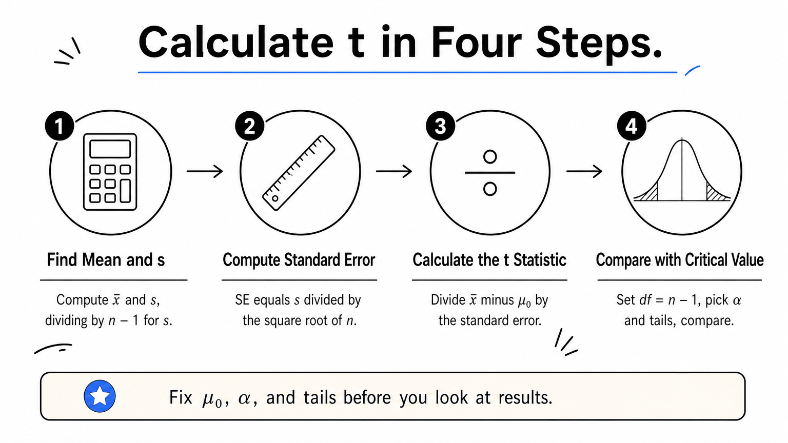
Fix μ₀, α, and the number of tails before you look at the results. Choosing them afterward lets you steer the outcome, even unintentionally.
t is the observed difference measured in standard errors, so always divide by s / √n, never by s alone.
Worked example: testing blood pressure against 120 mmHg
This example calculates t by hand for 10 resting systolic blood pressure readings against a reference of 120 mmHg. The data are hypothetical, chosen so the arithmetic stays visible.
The data and hypotheses
The 10 readings, in mmHg, are 124, 131, 118, 127, 135, 122, 129, 126, 133, and 125. You want to know whether the mean differs from 120 in either direction.

The null hypothesis is H₀: μ = 120. The alternative is H₁: μ ≠ 120, which makes this a two-tailed test. You set α = 0.05 before looking at the results.
The calculation
The readings sum to 1,270, so x̄ = 127.0. Deviations from the mean are −3, 4, −9, 0, 8, −5, 2, −1, 6, and −2. Squaring and adding them gives 240.
| Step | Calculation | Result |
|---|---|---|
| Sample mean | 1,270 ÷ 10 | 127.0 |
| Sum of squared deviations | 9 + 16 + 81 + 0 + 64 + 25 + 4 + 1 + 36 + 4 | 240 |
| Sample variance | 240 ÷ 9 | 26.67 |
| Sample standard deviation | √26.67 | 5.164 |
| Standard error | 5.164 ÷ √10 (3.162) | 1.633 |
| Mean difference | 127.0 − 120 | 7.0 |
| t statistic | 7.0 ÷ 1.633 | 4.29 |
| Degrees of freedom | 10 − 1 | 9 |
The decision
With 9 degrees of freedom and α = 0.05 (two-tailed), the critical value is ±2.262. Your t of 4.29 is larger than 2.262, so you reject the null hypothesis. The sample mean of 127.0 is significantly different from 120. In words: if the true mean were 120, a sample mean this far away would be very unlikely.
The decision rule is simple: reject H₀ when the absolute value of t exceeds the critical value for your df and α.
How to interpret your t statistic
A t value means little on its own. You interpret it with a critical value or p-value, a confidence interval, and an effect size, and you report all of them.
Critical values and tails
Critical values depend on degrees of freedom, so they shrink as your sample grows. These two-tailed values are standard t table entries:
| df | α = 0.05 | α = 0.01 |
|---|---|---|
| 9 | 2.262 | 3.250 |
| 19 | 2.093 | 2.861 |
| 24 | 2.064 | 2.797 |
| 30 | 2.042 | 2.750 |
| 60 | 2.000 | 2.660 |
If you stated a direction in advance, such as "the mean is higher than 120," use a one-tailed test. At df = 9 and α = 0.05 the critical value then drops to 1.833. Use this only when a result in the opposite direction would be meaningless to you. Otherwise stay two-tailed.
The p-value and the confidence interval
For t = 4.29 with 9 degrees of freedom, the two-tailed p-value is about 0.002. It is the probability of seeing a t this extreme or more extreme if H₀ were true. It is not the probability that H₀ is true.
The 95% confidence interval for the true mean is x̄ ± t_crit × SE, or 127.0 ± 2.262 × 1.633. That gives roughly 123.3 to 130.7 mmHg, and 120 sits outside it, which agrees with the test. Note that "95% confidence" corresponds to α = 0.05, not to a sample size. The sample size you need depends on the difference you want to detect, the variability, and the power you want. With only 10 readings, you can reliably detect large differences and little else.
Effect size and reporting
Significance does not tell you whether the difference matters. For a one-sample test, Cohen's d = (x̄ − μ₀) / s, which here is 7.0 ÷ 5.164 = 1.36. Common rules of thumb call about 0.2 small, 0.5 moderate, and 0.8 large, so this is a large effect. Treat those labels as rough guides and judge the difference against what is clinically or practically meaningful.
A compact way to report it is: t(9) = 4.29, p = .002, d = 1.36, 95% CI [123.3, 130.7]. State the sample size and the reference value in the sentence around it.
Report the t statistic, degrees of freedom, p-value, confidence interval, and effect size together, because each answers a different question.
Common mistakes and how to check your result
Most wrong answers come from a small set of errors in the standard deviation, the denominator, or the test choice. A quick check against software catches nearly all of them.
Mistakes that change the answer
- Dividing by s instead of s / √n. In the example that gives 7.0 ÷ 5.164 = 1.36, which is Cohen's d, not t.
- Using the population standard deviation. Excel's STDEV.P and NumPy's default np.std divide by n. Use STDEV.S in Excel, or ddof=1 in NumPy.
- Choosing a one-tailed test after seeing the data. That halves your p-value by hindsight.
- Applying the test to two groups. Independent groups need a two-sample test, and paired measurements need differences first.
- Treating a non-significant result as proof. Failing to reject H₀ means the data did not show a difference. It does not show that the mean equals μ₀.
Verifying with code or software
Python's SciPy reproduces the hand calculation in a few lines:
from scipy import stats

data = [124, 131, 118, 127, 135, 122, 129, 126, 133, 125]
result = stats.ttest_1samp(data, popmean=120)
print(result.statistic, result.pvalue)
You should see a t of about 4.287 and a p-value near 0.002, matching the table above. If your numbers differ, recheck the standard deviation first.
You can also let a tool do the work and still keep control. In PlotStudio AI you upload the CSV and ask for a one-sample t-test against 120. Verification Mode lets you review the proposed method and assumptions before anything runs, and you can read the generated Python afterward and compare it with this hand calculation. The software is an assistant. You still choose μ₀, judge the assumptions, and own the conclusion.
Always compute at least one result by hand, because a number you can reproduce is a number you can defend.
Using the formula on your own data
The one-sample t-test formula divides the difference between your sample mean and a reference value by s / √n, then checks that ratio against the t distribution with n − 1 degrees of freedom. If you set μ₀ and α in advance, verify the assumptions, and report the confidence interval and effect size alongside the p-value, the result is easy to defend.
Next time you have one column of measurements and one number to compare it to, work through the four steps once by hand, then confirm with software. If you want to run the test on your own dataset and inspect the code behind it, you can try PlotStudio AI free, with no credit card required.