Fitted coefficients can look tidy while the errors still move together. If the parameter table is the only thing you check, what did the model fail to absorb?
A Ljung Box test checks whether residuals from a fitted model still show autocorrelation at any lag up to a chosen h. The null says those autocorrelations are all zero. Rejecting it means some forecastable structure was left behind. A result that fails to reject is evidence the leftovers look like noise, not proof the specification is correct.
What the Ljung Box Test Checks in Your Residuals
Say you forecast monthly clinic visits with an ARIMA model. Coefficients are significant, and next month's point forecast looks sensible. The open question is what the fit threw away. Those one-step errors are the residuals, and they are the only series a Ljung Box test should see.
Think of the model as a sieve. A good sieve lets irregular grains through and holds back repeating clumps. White noise is the irregular grain. If a clump remains in the residuals, some lag still carries signal you could have modeled. The test does not crown a single lag. It asks whether any pattern slipped through anywhere from lag 1 to lag h.
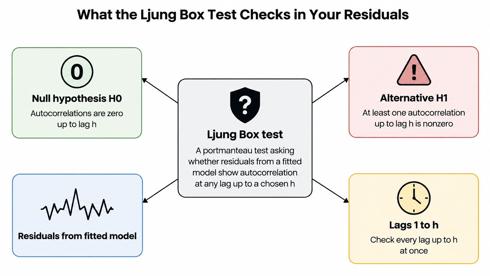
- Null, H0: autocorrelations at lags 1 through h are all zero.
- Alternative, H1: at least one of those autocorrelations is not zero, so some structure is still unmodelled.
- Input: residuals from an ARIMA, ARMA, regression with autocorrelated errors, or GARCH fit. Not the raw series.
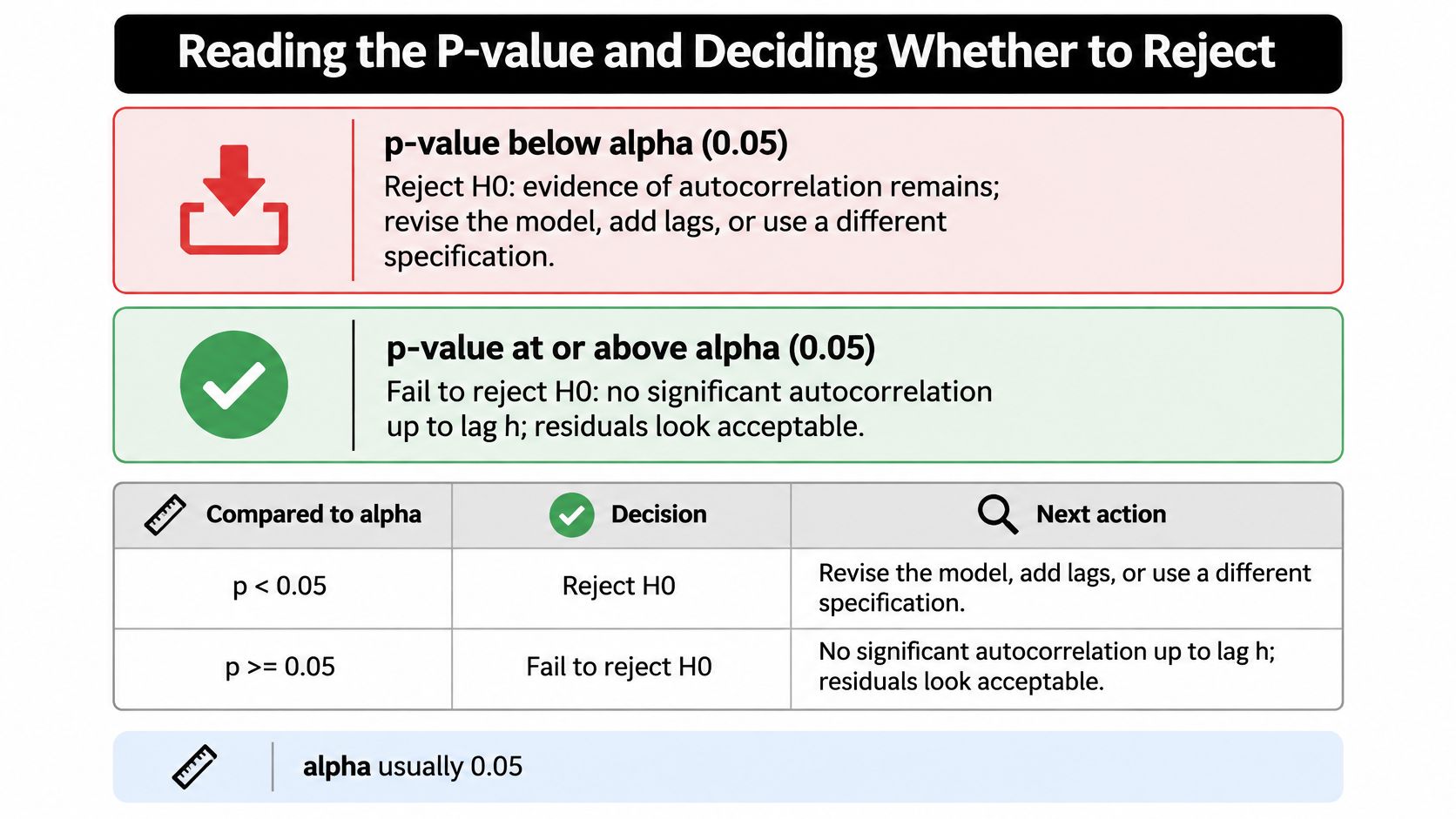
The statistic, usually called Q, grows as residual autocorrelation grows. Its reference is a chi-square distribution with h minus p minus q degrees of freedom. You reject H0 when the p-value falls below alpha, usually 0.05.
Do not feed the test the raw series. Visits, prices, and trial yields are expected to be autocorrelated, so a rejection there only rediscovers the signal. Econometrics, forecast validation, and residual checks in applied papers all use the test on what the model left behind. The lag-by-lag picture under that portmanteau result is what autocorrelation measures one lag at a time.
Write H0 and H1 for your own order, and name the residual series before you touch the raw data.
How the Q Statistic Adds Up Squared Autocorrelations
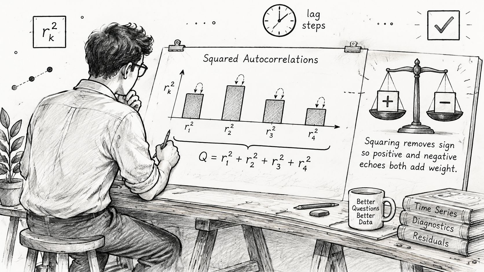
Each lag-k autocorrelation, written r_k, measures how strongly a residual lines up with the residual k steps earlier. A positive r_k means the errors keep the same sign. A negative r_k means they flip. Squaring drops the sign, so both kinds of echo land in the same pile. A quiet lag adds almost nothing. A loud lag adds a lot.
The weighted sum
The Ljung-Box form is
Q = n(n+2) Σ r_k² / (n−k), with k running from 1 to h.
n is the number of residuals. h is the last lag you chose to include. The weight n(n+2)/(n−k) is a small-sample correction. It is a bit larger at later lags, where fewer pairs are available, so a late echo is not ignored just because it is harder to estimate. Under the null, when residuals come from an ARMA(p, q) model, Q is referred to a chi-square law with h − p − q degrees of freedom.
Q is a running total of leftover structure, not a verdict on any single lag.
A numerical yardstick
Suppose n = 100, you test h = 10, and no AR or MA coefficients were estimated, so p and q are zero. The chi-square reference has 10 degrees of freedom. At the 5 percent level the critical value is about 18.3. A Q of 12 sits under that line and does not reject. A Q of 24 sits over it and does. After a real ARMA fit you spend degrees of freedom on the estimated terms before you read that tail. The statistic itself is unchanged. Only the yardstick moves.
A large Q means the combined echo across the lags you chose is bigger than chance usually produces when residuals are white noise. It does not name the guilty lag. That is why Q belongs beside an autocorrelation plot, not instead of one. If the plot is flat and Q is large, widen h and look again. If one bar sticks out and Q is small, you may be testing so many lags that one real spike is diluted.
Choosing Lags and Degrees of Freedom Correctly
| Setting | Lag h | Degrees of freedom | Notes |
|---|---|---|---|
| Short non-seasonal series, n = 40 | 8 (n/5) | 8 − p − q | Power is limited; keep h small |
| Non-seasonal series, n = 100 | 10 | 10 − p − q | Common default range |
| Long non-seasonal series, n = 1,000 | 7 (ln n) | 7 − p − q | Heuristic; confirm with sensitivity checks |
| Monthly data | 24 | 24 − p − q | Covers two seasonal cycles |
| Quarterly data | 8 | 8 − p − q | Covers two years |
Lag choice is a power choice. Too few lags and a seasonal spike never enters Q. Too many lags and a real spike is watered down by a long run of near-zero squares.
Short non-seasonal series. Use h = min(10, n/5). At n = 40 that is 8. You do not have enough pairs to support a long horizon, and extra lags mostly add noise.
Ordinary non-seasonal series. At n = 100, h = 10 is the usual working default. It is long enough to see short-run misspecification and short enough to keep power.
Long non-seasonal series. ln(n) is a heuristic, about 7 when n is 1,000. Treat it as a starting point and check nearby values, not as a law.
Seasonal series. Cover two cycles. Monthly data uses h = 24. Quarterly data uses h = 8. A test that stops at lag 10 can call a yearly pattern "fine."
The same residuals can stay acceptable as h moves. A 2025 study table reported simple Ljung-Box results at lags 10, 15, and 20, with test statistics of 6.194, 11.720, and 14.797 and p-values of 0.798, 0.700, and 0.788. The call did not flip.
Degrees of freedom after you estimate the model
Subtract the estimated autoregressive and moving-average orders. An ARMA(2, 1) tested at lag 10 has 10 − 2 − 1 = 7 degrees of freedom. Seasonal AR and MA orders come off the same way. Do not subtract a mean, drift, or intercept. Forget the subtraction and the chi-square reference is too wide, so a shaky model looks cleaner than it is.
Fix the lag set before you look at p-values. Then test three settings from the table and report the most conservative one, the result closest to rejection. Wider modeling choices sit in this guide to time series analysis methods.
Reading the P-value and Deciding Whether to Reject
Compare the p-value with alpha. At the usual 0.05, a smaller p-value rejects the null of no residual autocorrelation through lag h. A larger p-value means this test did not find enough joint signal to reject. High is the result you hope for, which is the reverse of a treatment test.
| P-value | Reading | Next action |
|---|---|---|
| Below 0.01 | Strong evidence of leftover autocorrelation | Revisit model order or add terms |
| 0.01 to 0.05 | Moderate evidence at common alpha levels | Inspect the ACF at the flagged lags |
| 0.05 to 0.10 | Not rejected at 5 percent; borderline | Check plots and sensitivity to lag choice |
| Above 0.10 | No evidence of autocorrelation at tested lags | Accept only with plots and other diagnostics |
Applied fits can land anywhere on that scale. A 2025 Scientific Reports table reported Ljung-Box Q-statistics at lag 9 ranging from 4.390 to 165.961 across six models, with p-values from 0.000 to 0.111. The same procedure separated a clearly misspecified fit from one this test would not reject.
A short reading routine
- Read every lag you precommitted to. One comfortable p-value does not cancel a rejection at a neighboring h.
- Look for clusters, not a single star. Massed significance at lags 12 and 24 is a seasonal miss, not a generic order to "add an AR term."
- Pick an action. Revise the order, keep the model, or re-specify. "Not rejected" is not the same word as "independent."
Short samples, and some awkward dependence patterns, have low power. Failing to reject does not prove the residuals are independent. For the limits of that number, see how to read a p-value.
A publication-ready line states alpha, each lag, Q, the degrees of freedom, and the p-value. This short video walks through that reporting habit with a residual series on screen.
Which Statistic to Report
Box-Pierce uses Q = n × Σ r_k². Ljung-Box inserts the weight n(n+2)/(n−k) on each squared autocorrelation. In small samples the Box-Pierce chi-square approximation is weaker, so the test has less power. As n grows, the two statistics converge, and a huge sample will not change your sentence much. A few hundred observations still can.
| Feature | Box-Pierce | Ljung-Box |
|---|---|---|
| Test statistic | Q = n × sum of r_k² | Q = n(n+2) × sum of r_k²/(n−k) |
| Reference distribution | Chi-square, h − p − q df | Chi-square, h − p − q df |
| Small-sample behavior | Weaker approximation, lower power | Better finite-sample approximation |
| Large-sample behavior | Nearly identical to Ljung-Box | Nearly identical to Box-Pierce |
| Software option | Available with boxpierce=True in statsmodels | Returned by default as lb_stat |
| Recommended use | Replicating older studies | Modern reporting and default choice |
statsmodels can return both. acorr_ljungbox puts the Ljung-Box statistic in lb_stat by default, and it adds Box-Pierce columns when boxpierce=True.
You will still meet Box-Pierce in older papers, textbooks, and legacy scripts. For any new analysis, report Ljung-Box. Mention Box-Pierce only when you are matching a published number. Before you compare two studies at the same lag, check which statistic each one printed. The values differ, sometimes enough to change a borderline call.
Running the Ljung Box Test in Python and PlotStudio AI
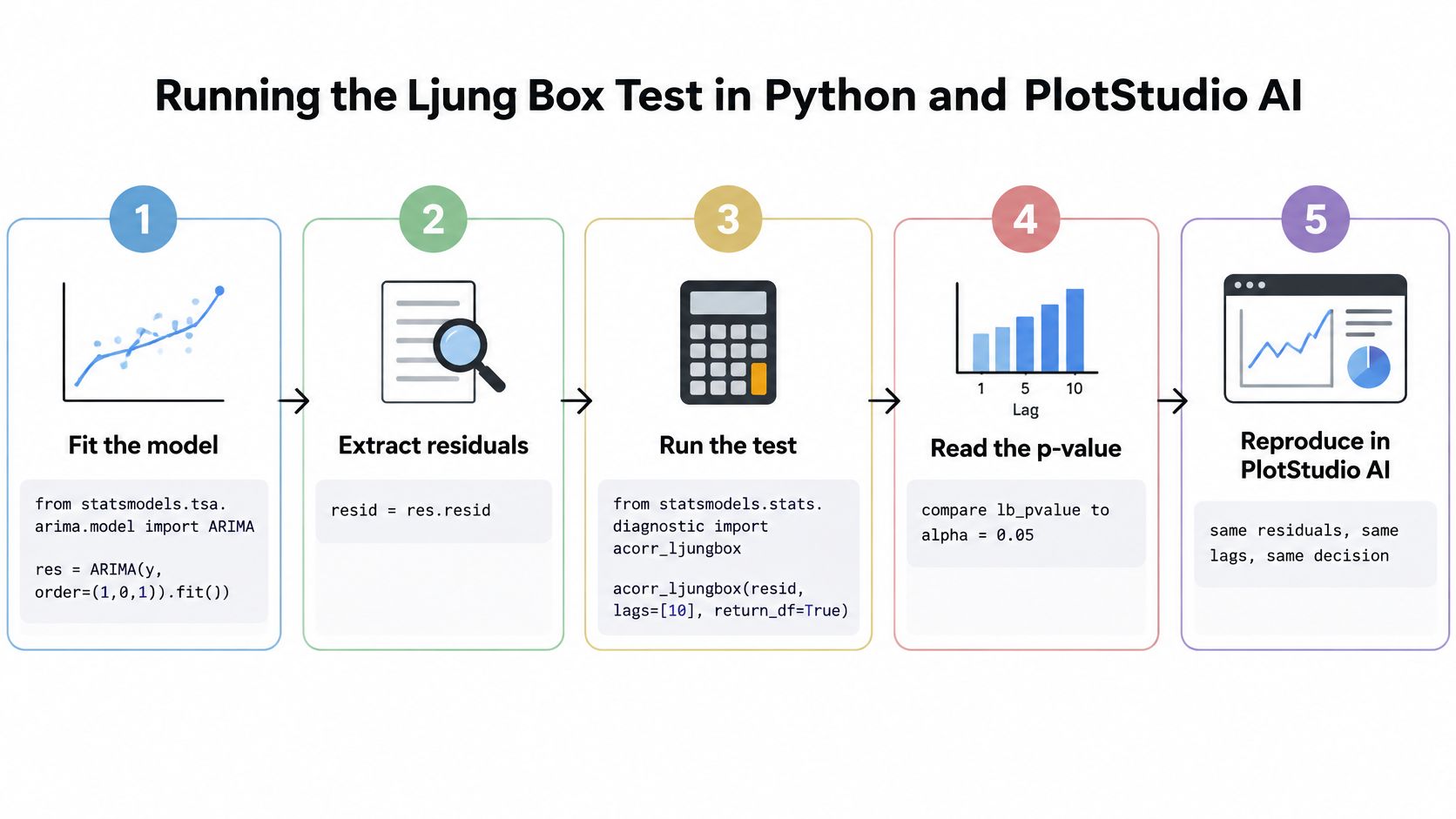
A reproducible run has six moves. Fit, extract residuals, test several lags, plot the residual ACF, repeat the test on squared residuals, and write down alpha, lags, degrees of freedom, and the decision.
- Fit.
from statsmodels.tsa.arima.model import ARIMA, thenres = ARIMA(y, order=(1,0,1)).fit(). - Extract.
resid = res.resid. Drop nothing unless you have a documented startup convention, and apply it the same way every time. - Test.
acorr_ljungbox(resid, lags=[10, 15, 20], model_df=2, return_df=True). Read lb_stat and lb_pvalue. For an ARMA(1, 1),model_df=2sets the reference to h minus 2. - Plot.
plot_acf(resid, lags=20)shows which lags carry the signal Q only totals. - Square. Run the same call on
resid ** 2so a variance pattern is not invisible to a levels test. - Record. Alpha, lags, degrees of freedom, Q, p-value, and whether you reject.
import numpy as np
from statsmodels.tsa.arima.model import ARIMA
from statsmodels.stats.diagnostic import acorr_ljungbox
from statsmodels.graphics.tsaplots import plot_acf

np.random.seed(7)
e = np.random.normal(size=120)
y = np.zeros(120)
for t in range(1, 120):
    y[t] = 0.6 * y[t - 1] + e[t]

res = ARIMA(y, order=(1, 0, 1)).fit()
resid = res.resid
print(acorr_ljungbox(resid, lags=[10, 15, 20], model_df=2, return_df=True))
plot_acf(resid, lags=20)
print(acorr_ljungbox(resid ** 2, lags=[10, 15, 20], return_df=True))
The simulated series is AR(1). The fitted order is slightly richer than the truth, which is a common real-world mismatch. You still judge the residuals, not the fact that the order "looks close."
A published multi-series table is read the same way. A 2025 study table reported Box-Ljung statistics for four residual series of 0.042763556, 0.231526123, 0.924857602, and 0.469479075, with p-values 0.836171125, 0.630394533, 0.336202749, and 0.493226916. Every p-value is above 0.05, so none of the four is rejected.
The same investigation without hand-written boilerplate
Agentic analytics is data analysis performed by AI agents that can plan an investigation, execute analytical steps with real tools and code, inspect intermediate results, revise the approach, validate outputs, and synthesize a complete analysis. An answer is an output. An analysis is an investigation. PlotStudio AI is an AI tool for researchers built around that pattern, not a claim to have invented it.
You upload the CSV and state the objective in plain English, for example "fit an ARIMA and run a Ljung Box test on the residuals at lags 10, 15, and 20." In Plan Mode you read the plan before it runs. The app executes Python locally, you inspect the generated code and the residual chart, and the work is saved as an Analysis Page with the statistics and the interpretation. Export is a Jupyter notebook if you want the script elsewhere. Hand-written Python still matters, and this Python path for statistical analysis is the habit the generated code should match.
Fix Pitfalls Before You Trust a Passing Test
A calm Ljung Box p-value only says that linear autocorrelation, inside the lags you chose, is small. Q pools those squared correlations and nothing else. Variance can still wander, a trend can remain, or the lag you needed can sit past h, and the p-value can still look fine.
| Pitfall | Symptom | Fix |
|---|---|---|
| Heteroskedastic residuals | Significant Q on squared residuals; variance shifts over time | Model variance with GARCH or transform the series |
| Nonstationary residuals | Slow ACF decay; p-values near zero at every lag | Difference the series or model the trend, then re-test |
| Wrong degrees of freedom | Overstated p-values after an ARMA fit | Subtract estimated p and q from h |
| Testing the raw series | Significant Q driven by the signal itself | Run the test on model residuals |
| Missed seasonality | Spikes at lag 12 or 24 in monthly data | Add seasonal terms and include seasonal lags |
| Too few observations for the lags | Unstable p-values across lag choices | Report several lags and shorten h |
Heteroskedasticity is the miss that looks like a pass. Time-varying variance works like a volume knob on an otherwise quiet signal: the levels show little linear autocorrelation, while the squares still move together. Test the squared residuals. If that Q is large, model the variance with GARCH or transform the series, then test again. The regression form of the same pattern is heteroscedasticity. After a GARCH fit, the series to check is the standardized residuals. The usual chi-square reference can be a little conservative, because the volatility path was estimated and the null is no longer pure white noise.
Nonstationarity looks different. The ACF decays slowly, and p-values sit near zero at every lag. Difference the series or put the trend in the model, then re-test the new residuals. A huge Q on an undifferenced trending series is the trend.
Two bookkeeping errors fake the result. Leave the estimated AR and MA orders in the degrees of freedom and the p-value after an ARMA fit is overstated. Test the raw series and Q rediscovers the signal the model was built to capture. Seasonal spikes at lag 12 or 24 in monthly data call for seasonal terms, with those seasonal lags inside h. When the sample is short for the lags you picked, p-values jump as h changes, so report several lags and shorten h.
Confirm a pass with residual plots, out-of-sample error, and stability across the three lags you fixed before seeing the p-values. Then run acorr_ljungbox on the residuals at those lags, test the squares, and record alpha, lags, degrees of freedom, and p-values.
PlotStudio AI can run that checklist on your file and keep a permanent analysis page for the question, with tables, charts, tests, and interpretation in one document. You can try PlotStudio AI free by signing up on its website. The trial is credit-based, and credits are used when analyses run.
Frequently Asked Questions About the Ljung Box Test
How do I run the Ljung Box test in R?
Call Box.test on the residuals, not on the raw series. A working call is Box.test(resid, lag = 10, type = "Ljung-Box", fitdf = 2). The fitdf argument is how many ARMA coefficients you estimated. The chi-square reference then uses h minus fitdf degrees of freedom, so the p-value does not pretend those coefficients were known before the fit. Leave fitdf at 0 only when you are testing a raw series you claim is white noise. On model residuals, a zero correction makes the test too willing to call a leftover quiet.
A rejection means squared autocorrelations from lag 1 through h are too large together. It does not name which lag, or which fix, caused that. A large p-value is evidence those lags look quiet under the corrected reference distribution. It is not proof the model is finished.
How does it differ from the Durbin-Watson test?
Durbin-Watson checks first-order autocorrelation in a regression residual. One number, one lag. A Ljung-Box Q sums squared autocorrelations from lag 1 through h, so a seasonal spike at lag 12 can move the statistic even when lag 1 looks fine. Keep Durbin-Watson as a fast screen after ordinary least squares. When the scientific question is whether a fitted time-series model left dependence across a whole horizon, report Ljung-Box at lags you fixed before looking at the p-values.
Can I apply it to panel data?
Apply it unit by unit. Residuals from different people, firms, or plots are separate ordered series. Pooling them into one column scrambles the lag index: time t for one unit can sit next to time 1 for the next, and the sample autocorrelation is no longer a time lag. A rejection is a clue about that unit's dynamics. Averaging those p-values does not turn the procedure into a panel test.
Download PlotStudio AI and run the residual check on a series you already know well, so you can see the plan, the Python, and the p-values side by side.