You've fitted a regression, the coefficient looks clear, and then the residual plot fans out like a megaphone. Heteroscedasticity in regression means your errors don't have constant variance, so your standard errors and tests may mislead you. PlotStudio AI can help you run the diagnostics and sensitivity checks, but you first need to know what each remedy changes.
What Heteroscedasticity Means in Plain Terms
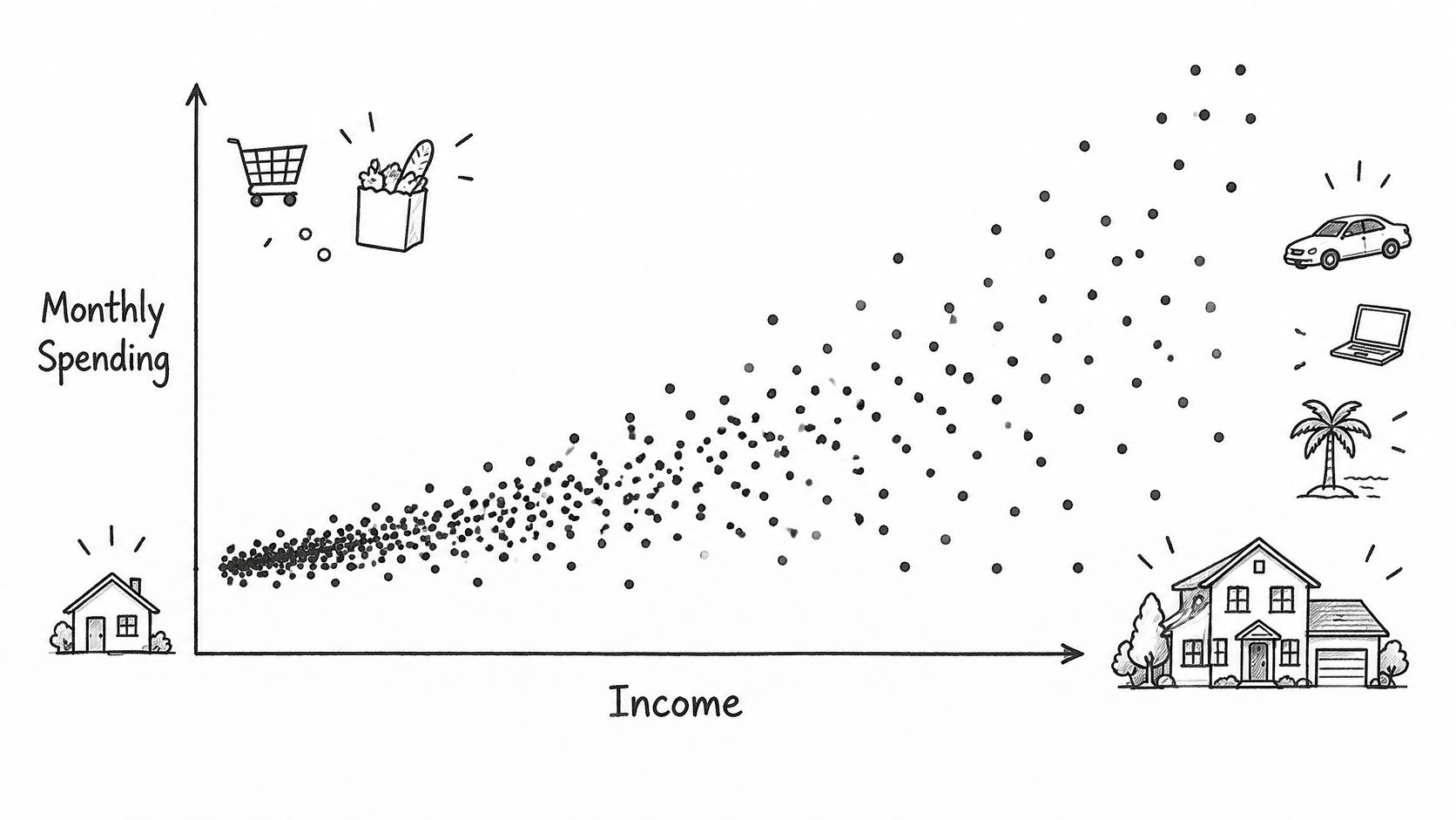
Say you survey households and regress monthly spending on income. Low income households cluster in a narrow spending band because rent and food leave little room to vary. High income households spread widely. Some save heavily, others spend freely, so the scatter fans out from left to right.
The regression line can still track average spending well. What's unequal is the scatter around that line.
The Definition in One Step
Heteroscedasticity means the variance of the error term changes across observations. Homoscedasticity means it's constant. Formally, heteroscedasticity is Var(u_i | x_i) = σ_i², where σ_i² varies by observation, instead of one common σ² for everyone.
The word comes from Greek roots, hetero for different and skedasis for dispersion. Think of a marksman whose shots cluster evenly at short range but scatter more at longer range. The aim hasn't shifted. The precision has.
Where It Usually Comes From
- Income scale: Larger budgets, firms, or farms have more room for large deviations in absolute terms.
- Measurement error proportional to size: A lab instrument or survey response that's off by a percentage produces bigger absolute errors for bigger values.
- Omitted variables that shift variance: A missing factor, such as household composition or management quality, can widen the spread for some groups more than others.
Notice what's not on that list. A fan shape doesn't automatically mean your predictors are wrong. It means the noise around your conditional mean isn't uniform, and that distinction drives every decision that follows.
Heteroscedasticity does not move the line; it changes how much you should trust the line's precision.
That sentence is worth keeping in front of you. Many researchers panic and rebuild the whole model when they see a funnel. Others ignore it because the coefficients look stable. Neither reaction is right, because the damage is specific, and so is what survives.
What Breaks in OLS Inference and What Survives
Here's the bottom line first. When your mean model is correct, OLS coefficients remain unbiased and consistent under heteroscedasticity. What fails is efficiency and the standard errors you'd normally use to judge those coefficients.
OLS stops being the best linear unbiased estimator. Another estimator that downweights noisy observations can estimate the same coefficients more precisely. You're not getting the wrong answer on average. You're getting a noisier answer than you needed to.
Why the Textbook Formula Fails
The classical variance formula, σ²(X'X)⁻¹, assumes one common σ². Once each observation has its own σ_i², that formula is the wrong description of your sampling uncertainty. Every t-test, F-test, and confidence interval built on it inherits the error.
Say a classical standard error comes out too small. Your t-statistic inflates, your 95% interval narrows, and you reject true null hypotheses more often than the nominal 5% rate. You'd report findings that aren't there.
The direction isn't fixed, and that's the trap. Classical standard errors can be too small or too large, depending on whether high variance observations sit at influential positions in your design. You can't assume you're being conservative. Prediction intervals suffer too, because a single width can't be right where variance is small and where it's large. This variance problem is distinct from correlated errors, which is why it's useful to separate it from autocorrelation in regression errors when you diagnose a model.
R-squared doesn't rescue you either. It remains a valid descriptive summary of fit in your sample, but it tells you nothing about whether the variance structure is constant.
| Property | Homoscedastic errors | Heteroscedastic errors |
|---|---|---|
| Coefficient estimates | Unbiased and consistent | Still unbiased and consistent when the mean model is correct |
| Efficiency | OLS is the best linear unbiased estimator | OLS is no longer efficient; weighted estimators can do better |
| Classical standard errors | Valid | Biased, can be too small or too large |
| t-tests, F-tests and confidence intervals | Nominal size and coverage | Size and coverage distortion |
| Prediction intervals | Correctly calibrated | Miscalibrated where variance differs |
| R-squared | Valid descriptive measure | Still descriptive; does not reveal variance structure |
Read the first row and the third row together. That pairing is the whole problem in miniature.
How to Detect It with Plots and Tests
Start with plots, not tests. A test gives you a p-value. A plot shows you where the variance changes, which is what you need to choose a remedy.
Three Plots to Make First
Plot residuals against fitted values and look for a funnel or wedge that widens or narrows. Then plot residuals against each regressor, because variance may track one predictor rather than the fitted mean. Finally, make a scale-location plot of the square root of absolute standardised residuals against fitted values. A rising or falling trend there signals changing spread.
The three panels below summarise what you're looking for in each view.
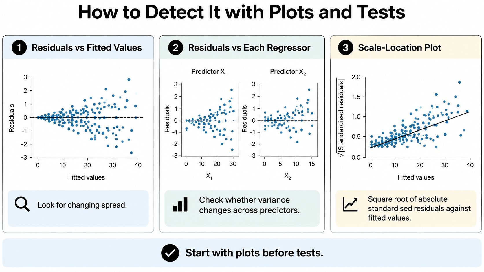
Read shape carefully. A funnel points to unequal variance, while a curved band points to a misspecified mean, which is a different problem needing a different fix. These plots sit inside a broader set of regression diagnostics that you should run together rather than in isolation.
Be cautious in small samples. Random scatter often looks structured when you have few points, and one or two outliers can fake a funnel.
Then Run Formal Tests
| Test | Null hypothesis | Auxiliary model | Practical note |
|---|---|---|---|
| Breusch-Pagan | Variance does not depend on the regressors | Squared residuals on the regressors; LM = n × R² | Use the studentised (Koenker) version when errors are not normal |
| White | Variance is constant, with no dependence on regressors, their squares or cross-products | Squared residuals on regressors, squares and cross-products | No functional form assumed; degrees of freedom rise quickly with many regressors |
| Goldfeld-Quandt | Equal variance across two ordered subsamples | Separate regressions after dropping central observations | Needs a sort variable you can justify before looking at the data |
Interpret every p-value by stating the null hypothesis, your chosen alpha, and your sample size. A rejection tells you variance isn't constant, but it doesn't reveal the form of the pattern. A non-rejection in a small sample is weak evidence of constancy, not proof, because the test may lack power.
Don't run several tests and report only the one that agrees with you. Report all of them. Disagreement between Breusch-Pagan and White is itself information about the shape of the variance function.
Practical rule: A significant test with a flat residual plot, or a clear funnel with a non-significant test, means you should investigate further, not pick the answer you prefer.
Use this three step checklist. First, plot the residuals three ways. Second, run the tests and report them all. Third, ask whether a remedy would change your conclusions for the coefficient you care about. If it wouldn't, say so and show it.
How to Fix It with Robust, Transformed and Weighted Models
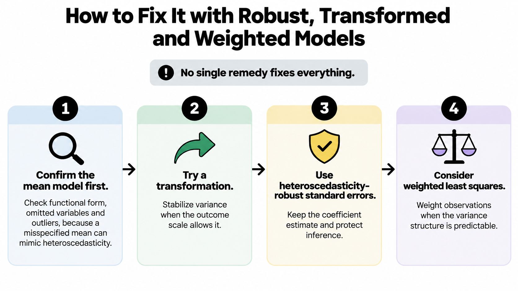
A widening residual funnel can come from unequal error variance, a poorly specified mean, or both. Choose a remedy based on the coefficient you want to estimate and the purpose of the model. Each option changes something different.
Six Steps in Order
- Check the mean model first. Review its functional form, omitted variables, and influential observations. A misspecified mean can create residual patterns that resemble changing variance. Variance corrections do not fix that misspecification.
- Name the estimand. Decide whether you want an effect on the outcome's original scale or a proportional effect. A transformation can change the question your coefficient answers.
- Use heteroscedasticity-consistent standard errors when the OLS coefficients are your target. HC1 is a common choice; HC3 is often used in smaller samples. These adjustments change the estimated uncertainty, not the OLS coefficients or fitted values. See this guide to heteroscedasticity-robust standard errors for how the HC variants differ.
- Transform the outcome if its scale and interpretation justify it. Logging a strictly positive outcome may help when its spread grows with its level. The model then describes effects on a transformed scale, often interpreted proportionally.
- Use weighted least squares only with defensible weights. Weights should be proportional to the inverse of the error variance. WLS changes the coefficient estimates as well as their precision; incorrect weights can make the estimates less useful.
- Consider feasible GLS when the variance pattern must be estimated. Estimate the variance function from residuals, then use it to construct weights. Because those weights are estimated, their uncertainty also matters.
Standard errors adjusted for heteroscedasticity are an inference adjustment, not a repair to the whole model. They leave the OLS coefficients, fitted values, and conditional mean unchanged. In small samples or with a few highly influential observations, heteroscedasticity-consistent corrections can be unreliable. Compare conventional, HC2, HC3 or HC4, bootstrap, and weighted results for the coefficient or contrast you care about rather than relying on one default.
This short walkthrough shows the remedy sequence applied to a fitted model.
| Remedy | What it changes | Main requirement | Main risk |
|---|---|---|---|
| Robust (HC) standard errors | Standard errors only; coefficients stay OLS | No variance model needed | Can be unreliable in small samples or with high-leverage observations; does not improve efficiency |
| Log or other transformation | Outcome scale and coefficient interpretation | Transformation suits the outcome and research question | The coefficient refers to a different estimand |
| Weighted least squares | Coefficient estimates and their precision | A credible model for the variance and weights | Incorrect weights can be worse than unweighted OLS |
| Feasible GLS | Coefficient estimates, using an estimated variance function | Variance function can be estimated from residuals | Estimated weights add uncertainty |
For each remedy, ask what it changes and what it leaves alone. If your goal is inference on an OLS coefficient, standard errors adjusted for heteroscedasticity may be enough. If your goal is more efficient estimation under a credible variance model, weighting may be appropriate. A transformed outcome answers a different question, so use it only when that change in interpretation fits your research aim.
Worked Example and Simulation in Python and R
Suppose measurement error grows with the level of a predictor. A simulation makes the consequences visible because the true slope is known. Set n = 500, draw (x) from Uniform(1, 10), and generate (y = 2 + 3x + e), where (e) is normal with standard deviation (0.5x). The error variance therefore grows with (x), and the true slope is 3.
Python with statsmodels
import numpy as np
import statsmodels.api as sm
from statsmodels.stats.diagnostic import het_breuschpagan, het_white

rng = np.random.default_rng(42)
x = rng.uniform(1, 10, 500)
y = 2 + 3*x + rng.normal(0, 0.5*x)
X = sm.add_constant(x)

ols = sm.OLS(y, X).fit()
print(het_breuschpagan(ols.resid, X))
print(het_white(ols.resid, X))

ols.get_robustcov_results(cov_type="HC3")
print(ols.summary())

print(sm.WLS(y, X, weights=1/x**2).fit().summary())
The fixed seed makes the run reproducible. The Breusch-Pagan and White tests use residuals from the OLS fit. HC3 changes the standard errors, not the OLS coefficients. The WLS weights (1/x^2) match the inverse of the error variance, since the error standard deviation is (0.5x). For more on the surrounding workflow, see this guide to Python for statistical analysis.
R with lmtest and sandwich
set.seed(42)
x <- runif(500, 1, 10)
y <- 2 + 3*x + rnorm(500, 0, 0.5*x)
fit <- lm(y ~ x)

lmtest::bptest(fit)
lmtest::coeftest(fit, vcov = sandwich::vcovHC(fit, type = "HC3"))
summary(lm(y ~ x, weights = 1/x^2))
lm() fits OLS, and bptest() runs the Breusch-Pagan test. coeftest() with vcovHC(type = "HC3") reports HC3 inference for the same OLS coefficients. The final model uses the variance-based weights.
Check Coverage, Not Just One Run
A single simulated dataset cannot show how often an interval procedure succeeds. Repeat the simulation 2,000 times, form a 95% interval for the slope in each run, and count the share of intervals that contain the true slope of 3. Compare classical OLS, HC3 OLS, correctly weighted WLS, and WLS with the deliberately incorrect weights (1/x).
| Estimator | 95% interval coverage of slope 3 | Efficiency |
|---|---|---|
| OLS with classical standard errors | Below 95% | Lower than correctly weighted WLS |
| OLS with HC3 standard errors | Approximately 95% | Lower than correctly weighted WLS |
| WLS with correct weights | Approximately 95% | Highest under this variance model |
| WLS with wrong weights and conventional standard errors | Below 95% | Not guaranteed |
| OLS with HC3 under a misspecified mean | Does not target the true slope | Not applicable |
These are typical simulation outcomes, not guaranteed results for every random seed. The comparison separates two goals: coverage concerns uncertainty estimates, while efficiency concerns how precisely an estimator uses the data.
Add one deliberate mistake: generate (y) with a curvature term, then fit a straight line and apply HC3. HC3 adjusts uncertainty around the fitted linear relationship. It does not correct the mean model, so the intervals can be well calibrated for a coefficient that does not represent the true slope.
Choosing a Remedy for Your Research Question
A researcher estimating how a training program affects wages may want a defensible coefficient, while a planner forecasting next year's costs may care more about prediction accuracy. Heteroscedasticity does not decide the remedy by itself. The goal of the model does.
For coefficient inference in a moderate cross-section, HC3 standard errors adjust uncertainty estimates while leaving the OLS coefficients unchanged. If a credible variance pattern is available, weighted least squares (WLS) or feasible GLS may improve efficiency by giving observations different weights. Those methods change how the model is estimated, so the resulting coefficient can differ from OLS.
A log transformation can suit a positive outcome whose spread grows with its level. It changes the scale and interpretation of the model: effects become proportional rather than additive. Recheck residuals on that scale. When variance depends on unobserved factors, heteroscedasticity-consistent standard errors and sensitivity analysis avoid imposing a variance model that the data do not support.
Clustered and Panel Data
Observations within the same firm, school, or field plot may share shocks. Cluster-adjusted standard errors account for within-cluster dependence, including unequal variance, while leaving the fitted coefficients unchanged. They work best with enough clusters; with few clusters, a wild cluster bootstrap can provide an alternative for inference.
For panel data, fixed effects account for stable differences between units, while clustered errors address dependence within units. These choices do not, by themselves, explain how variance changes over time. To model variance explicitly, specify log σᵢ² as a function of observed variables, estimate it, and use the fitted variances to construct weights. Then check whether conclusions hold with heteroscedasticity-consistent standard errors.
If the research question concerns conditional quantiles rather than the conditional mean, quantile regression estimates effects at different points of the outcome distribution. That changes the estimand, not just the standard errors.
Heteroscedasticity can coexist with multicollinearity, influential observations, missingness, time variation, or autocorrelation. Separate these problems before choosing a remedy: changing the variance model will not correct coefficient drift or collinearity. A 2025 study in Communications in Statistics reports that heteroscedasticity-adjusted ridge estimators can outperform conventional alternatives when multicollinearity is high, across low, high, and severe heteroscedasticity settings. Ridge estimation also changes the coefficient estimates, so it is not a standard-error correction.
| Research situation | First choice | Why |
|---|---|---|
| Coefficient inference, cross-section, moderate sample | HC3 standard errors | Adjusts inference without changing the OLS coefficient |
| Prediction with a credible variance pattern | WLS or feasible GLS | Uses the variance pattern in estimation and may improve efficiency |
| Positive outcome whose spread grows with its level | Log transform, then check residuals | Changes the outcome scale and makes effects proportional |
| Panel data or repeated observations | Cluster-robust standard errors at the unit level | Allows dependence within units |
| Small sample or high leverage | HC3 or bootstrap, reported with sensitivity checks | Inference can be sensitive to sample size and influential observations |
| Variance driven by unobserved factors | Robust standard errors plus sensitivity analysis | Avoids relying on an unsupported explicit variance model |
Choose remedies by what they change: standard-error corrections alter uncertainty, weighting alters estimation, and transformation alters the scale and interpretation. Compare the target coefficient under appropriate alternatives, then report whether its sign and statistical significance remain consistent.
Confirm the Remedy Before You Report Results
A coefficient can keep the same value while its uncertainty changes. Before reporting a remedy, check that it fits your research question and show how your conclusion responds to reasonable alternatives.
- Write the estimand in one sentence. State what quantity you want to estimate and whether it must remain on the original outcome scale.
- Save the residual plots and test output. Keep them with the analysis so readers can see what prompted the remedy.
- Compare the target coefficient across methods. Include classical and HC3 standard errors, then add a weighted model or bootstrap when appropriate. Separate changes to the coefficient from changes to its uncertainty.
- Name the standard-error method in every table note. Specify HC3, clustering by school, or the bootstrap procedure. “Robust” alone does not identify the method.
- Report how the conclusion changes. Describe differences in sign, magnitude, and statistical significance across specifications.
- Keep the code. Another analyst should be able to reproduce the choices and results.
Use this final checklist before sharing the results.
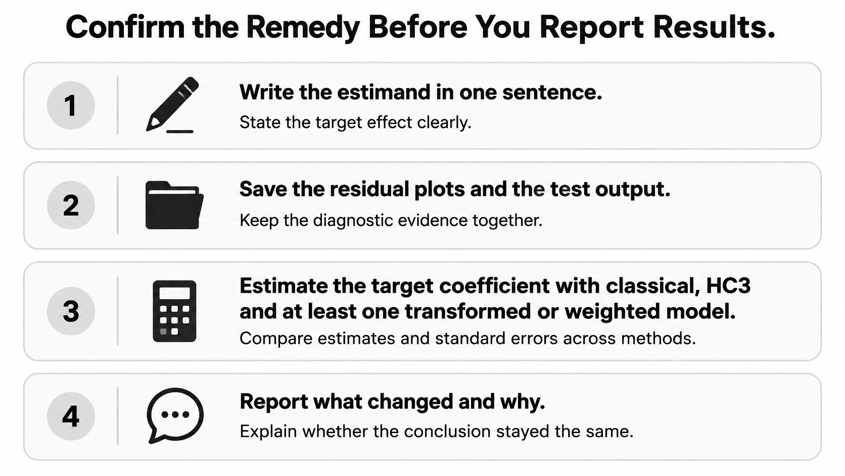
An auditable analysis records the steps from residual checks to the reported model. The record helps another analyst distinguish a change in standard errors from a change in the model or estimand.
PlotStudio AI saves each step in an Analysis Page with the generated Python. Its cleaner documents transformations, including rows dropped, imputations, and recodings, so the output can be reviewed.
PlotStudio AI can keep each step of a heteroscedasticity check saved as a reproducible analysis with its code.
Frequently Asked Questions
Does Heteroscedasticity Bias OLS Coefficients
No. When the mean model is correct, coefficients stay unbiased and consistent. What's wrong is the classical standard errors, and therefore your t-tests and confidence intervals.
Are Robust Standard Errors Always Enough
They correct inference on coefficients only. They don't restore efficiency, improve prediction intervals, or fix a misspecified conditional mean. If prediction is your goal, you need to model the variance.
Should I Report Breusch-Pagan or White
Report both. Breusch-Pagan assumes a linear variance function in the regressors, so it has more power when that's right. White needs no functional form, but it consumes degrees of freedom quickly as regressors and cross-products multiply.
How Large Must the Sample Be for the Tests to Work
Power rises with n, and there's no threshold where a test suddenly becomes trustworthy. In small samples, treat a non-rejection as weak evidence of constant variance, not proof, and lean on your residual plots.
When Should I Log-Transform Instead of Weighting
Use a log transform when the spread of a strictly positive outcome grows with its level and a proportional effect is the estimand you want. Use weighted least squares when you have a credible variance model and you want to keep the original-scale coefficient.