Among Management Science articles using statistical software from 2019 to 2023, Stata appeared in 60%, according to a study of research software trends. Stata for data analysis combines data preparation, statistical models, graphics, and reporting in a command-driven environment. Its practical strength is an inspectable script that records how raw observations became a research result.
What Stata Is and Who Relies on It
Say an education researcher wants to examine whether school funding is associated with student achievement. They have assessment files, school characteristics, and repeated observations over time. Stata lets them combine those files, inspect missing values, estimate a panel model, and produce a table without moving between unrelated applications.
Stata is commercial statistical software from StataCorp. Its first official release arrived in January 1985, according to StataCorp's history of Stata. The useful distinction today isn't its age, but its integrated approach to managing data and estimating models.
Commands make the work inspectable
Each operation can be expressed as a command. summarize score describes a variable; regress score funding estimates a linear relationship. Save those operations in a do-file, and another analyst can inspect the sequence rather than reconstruct it from screenshots.
Menus provide an accessible starting point, but a saved analytical workflow is more useful than a collection of menu results. Researchers can discuss the same commands, check their assumptions, and identify where their results diverge.
Adoption isn't the same as suitability
The opening adoption figure describes software mentions in one journal, not universal market share. Papers can mention several tools, so those mentions shouldn't be treated as mutually exclusive purchasing decisions.
Stata is relevant to economists, political scientists, sociologists, epidemiologists, clinical researchers, and education and policy analysts. Nevertheless, disciplinary familiarity alone isn't enough reason to choose it.
First check: Match the software to your research design, available hardware, institutional access, and need for auditable scripts, not simply to what colleagues use.
The Stata Workflow From Raw Files to Analysis Sample
A defensible model starts with a defensible dataset. Stata's feature overview documents importing, transformations, merges, appending, labeling, and other preparation operations within the same environment.
The workflow below separates loading a file from establishing that it's suitable for analysis.
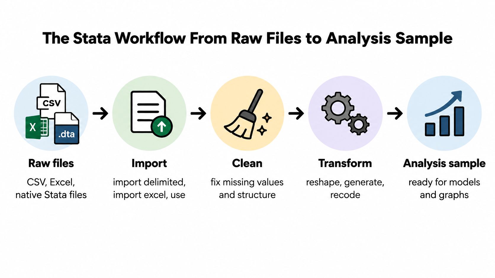
Stata workflow stages and the commands that drive them
| Stage | Core Stata commands | Output to check before moving on |
|---|---|---|
| Import | import delimited, import excel, use |
Raw data loaded with variable types confirmed |
| Inspect | describe, codebook, misstable summarize |
Missingness and types documented per variable |
| Clean | drop, replace, label variable, assert |
Cleaning steps recorded with row counts dropped |
| Merge | merge 1:1, merge m:1, append |
_merge tabulated; no unexpected duplicate keys |
| Derive | generate, egen, recode |
Analysis variables labeled and checked against codebook |
| Explore | summarize, tabulate, histogram, scatter |
Distributions and outliers reviewed before modeling |
| Estimate | regress, logit, xtreg, stcox |
Estimates, standard errors, and diagnostics saved |
Inspect before changing anything
Use import delimited for CSV files, import excel for workbooks, and use for native Stata files. Confirm that dates, identifiers, and numeric measurements have the intended types. A school identifier with leading zeros shouldn't become an ordinary measurement just because it contains digits.
Next, inspect the codebook and missingness. Distinguish unavailable measurements from values representing inapplicable questions or skipped visits. The data-profiling guide provides a useful framework for documenting those checks before cleaning.
Don't automatically delete unusual observations. Compare them with plausible ranges, source records, and collection rules first. Use assert to encode conditions that must hold, and isid schoolid year when each school-year combination should uniquely identify an observation.
Combine files without changing the unit of analysis
For the education example, school characteristics might contain one record per school, while assessment data contain repeated school-year records. That calls for a many-to-one merge on the school identifier, not an arbitrary join.
Stata's declared merge relationships check key uniqueness. A merge 1:1 doesn't accept nonunique keys; it stops when its uniqueness requirements fail. Other join operations can expand rows, so establish the intended relationship before combining files.
After a merge, inspect _merge before deciding which observations to retain. Unmatched doesn't automatically mean unusable. Investigate whether unmatched records reflect different coverage, identifier errors, or a legitimate sample restriction.
Use append when files represent additional observations with compatible variables. Use generate, egen, and recode only after confirming the meaning of the source fields.
For a visual introduction to working in Stata, this video can accompany hands-on practice.
Finally, explore distributions and relationships before fitting a model. Record observation counts after importing, merging, cleaning, and applying exclusions. That makes every change in the analysis sample visible.
Which Stata Command Fits Your Research Design
| Research design | Declare first | Core estimation commands |
|---|---|---|
| Cross-sectional continuous outcome | None | regress |
| Binary outcome | None | logit, logistic for odds ratios |
| Ordered or count outcome | None | ologit, poisson, nbreg |
| Panel data | xtset panelid timevar |
xtreg, fe; xtreg, re |
| Time-to-event outcome | stset time, failure(event) |
stcox, streg |
| Time series | tsset timevar |
arima, var |
| Instrumental variables | None | ivregress 2sls |
These are starting points, not automatic model-selection rules. Stata's statistical overview distinguishes fitting models from evaluating assumptions, drawing inference, and interpreting estimates. Choosing a command addresses only part of that work.
Panels require a unit, a clock, and a dependence model
xtset schoolid year tells Stata which observations belong to the same school and how they're ordered. It doesn't decide whether fixed effects, random effects, or another estimator fits your question.
Fixed effects absorb time-invariant unobserved differences between units. They don't resolve time-varying confounding, reverse causality, or measurement error. Conventional random-effects models assume the unit-specific effects are uncorrelated with the included covariates.
Stata's panel-data documentation describes these estimator families and inference options. Choose the clustering level from the design, including treatment assignment and plausible error dependence, rather than accepting a default standard error.
For example, repeated measurements within schools aren't independent just because each occupies a different row. The panel-data analysis guide helps distinguish within-unit comparisons from between-unit comparisons.
Survival models require a precise event definition
For time-to-event data, define the event, time origin, censoring, and entry rules before estimation. stset time, failure(event) is a simple right-censored declaration, not a universal declaration for every survival dataset.
Stata's survival-analysis documentation covers censoring, delayed entry, repeated-event settings, and parametric alternatives. Interval-censored outcomes require appropriate declarations and estimators, rather than ordinary stcox applied mechanically.
After a Cox model, use estat phtest where applicable to assess proportional hazards, alongside graphical and substantive checks. A proportional-hazards model concerns relative instantaneous event risk; an accelerated-failure-time model concerns acceleration or delay in event timing. Those interpretations aren't interchangeable.
Instruments require an argument beyond syntax
ivregress 2sls requires a defensible instrument, not merely a variable correlated with exposure. Inspect first-stage results with estat firststage, but recognize that relevance diagnostics don't establish the exclusion restriction.
A correctly executed command can estimate the wrong quantity precisely. The research design determines whether a causal interpretation is defensible.
Report effect sizes and confidence intervals, address multiple testing when relevant, and compare plausible specifications. An E-value can support sensitivity analysis in suitable effect-measure settings, but it isn't a general diagnostic for every model or source of bias.
Reproducible Do-Files and Interactive Menus
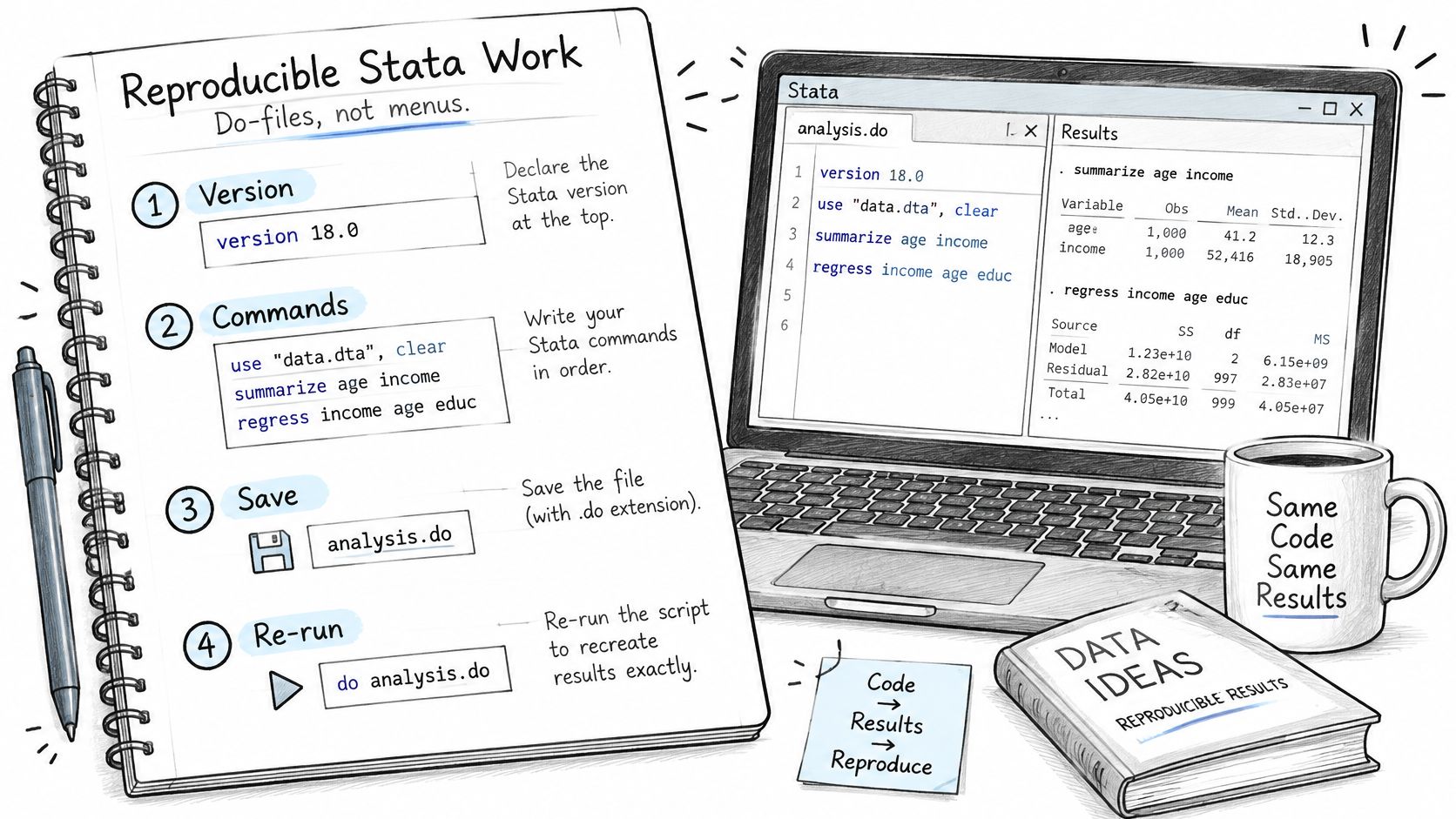
A do-file should explain how to regenerate the result, not merely preserve the final regression. Stata's reproducibility documentation recommends a version statement so commands are interpreted using the specified language behavior, including the example version 19.5.
Build an executable record
- Declare the version. Use the version appropriate to the environment you're documenting. A version statement doesn't install commands unavailable in an older installation.
- Open a log. Use
log usingwith a dated filename for retained runs, so you can distinguish outputs from different executions. - Control random operations. Set a seed before sampling, simulation, imputation, or bootstrap procedures. Record the procedure and settings too.
- Protect raw files. Read the source dataset without overwriting it. Save derived data separately and document where the source came from.
- Separate analytical stages. Label cleaning, validation, estimation, diagnostics, and reporting. Make exclusions and variable definitions explicit.
- Generate outputs programmatically. Use
putdocx,putexcel, or the appropriate reporting command rather than manually editing published values.
This illustrative snippet assumes a raw survey file containing an income variable. Its seed is an example setting, not a study result.
version 19.5
log using "analysis.log", text replace
set seed 20260101

use "raw_survey.dta", clear

generate log_income = ln(income) if income > 0 & !missing(income)
label variable log_income "Natural log of positive income"

putdocx begin
putdocx paragraph
putdocx text ("Summary of derived income variable")
summarize log_income
putdocx table summary = (2, 2)
putdocx table summary(1, 1) = ("Variable")
putdocx table summary(1, 2) = ("Mean")
putdocx table summary(2, 1) = ("Log income")
putdocx table summary(2, 2) = (r(mean))
putdocx save "summary.docx", replace

log close
The example uses replace for repeatable practice runs. Archive important outputs separately if you need to preserve each run.
Use menus to learn, scripts to retain
Menus issue commands that beginners can inspect in the command history and adapt into a do-file. Stata's interface overview also describes programmable workflows and frames for managing multiple datasets simultaneously.
A dynamically updated document isn't proof of complete provenance. Record data versions, user-written package dependencies, and any external processing alongside the script. A research-reproducibility checklist helps extend that record beyond the exported table.
Audit test: Can a colleague explain every exclusion and derived variable without asking the original analyst?
Stata License Costs for 2026
Listed Stata license prices in 2026
| License | Listed price (2026) | Term or condition |
|---|---|---|
| Stata/MP4 annual license | $995, listed by StataCorp's license-options page | Annual term, individual purchase |
| Stata/BE network license, 196 users | $11,763, listed by StataCorp's government network-license page | Two-year maintenance |
| Stata/MP4 annual license, student lab | $995, listed by StataCorp's educational lab-license page | Annual license listed for lab purchasing |
The individual annual listing is a recurring term, not a perpetual entitlement. The network listing covers maintenance for the stated deployment, not an individual seat. The student-lab listing belongs to a separate purchasing context and shouldn't be assumed to establish every student's personal license price.
Budget for the actual deployment
Before purchasing, check with your library, department, or IT team for institutional access. Confirm whether access covers your own computer, shared lab machines, remote sessions, or only a managed institutional environment.
Also confirm the edition, current terms, and whether StataNow updates are included. A license that fits a teaching lab may not fit a research group running unattended analyses on shared infrastructure.
R and Python are free and open source, so their software-access cost differs from Stata's. Your practical comparison should also include training, package maintenance, computing resources, and the work needed to reproduce an existing disciplinary workflow.
- Individual research: Check personal installation rights and access after graduation or contract completion.
- Shared labs: Confirm permitted users, concurrent access, and administration responsibilities.
- Application projects: Separate statistical software costs from interface development and hosting.
If your project also needs a custom application around its analysis, AppJet's option to browse full-stack development plans provides a separate budgeting reference. Application development isn't a substitute for a statistical license, and the two shouldn't be bundled mentally into the same expense.
Stata Compared With R, Python, SAS and PlotStudio AI
Choose by methodological fit, inspectability, and maintenance, not by which interface produces an answer fastest. This comparison distinguishes lower entry friction from the expertise needed to validate a study.
Stata compared with R, Python, SAS and PlotStudio AI
| Criterion | PlotStudio AI | Stata | R | Python | SAS |
|---|---|---|---|---|---|
| Core interface | Plain-English questions; generated Python shown | Menus plus command line | Scripts | Scripts and notebooks | Programs and menus |
| Multi-step investigation | Plans, runs, and revises analytical steps | User-scripted sequence | User-scripted sequence | User-scripted sequence | User-scripted sequence |
| Panel and survival methods | Local Python; estimator visible in code | Built-in xt and st commands |
Packages such as plm and survival |
Packages such as statsmodels and lifelines |
Procedures such as PROC PHREG |
| Reproducibility | Code, methodology, and Jupyter export per Analysis Page | Do-files with version statement | Scripts and R Markdown | Scripts and notebooks | Programs and logs |
| Local execution | Code runs on the user's machine | Desktop installation | Local | Local | Local or server |
| Cost | Credits or bring-your-own-key; check current terms | Paid license | Free, open source | Free, open source | Paid license |
| Learning curve for non-programmers | Low entry friction; validation still requires expertise | Moderate | Steep for script-first work | Steep for script-first work | Moderate to steep |
The visual comparison provides a compact reference, but method availability and execution records matter more than chart appearance.
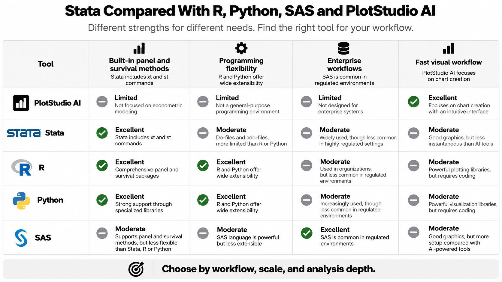
Established methods versus custom programming
Keep Stata when collaborators already maintain validated econometric or survival pipelines and reviewers expect inspectable do-files. Its integrated command families reduce the amount of infrastructure the analyst must assemble, although they don't remove the need to understand the estimator.
Choose R or Python when the project requires extensive custom programming or close integration with a broader software ecosystem. Package selection creates responsibilities: inspect defaults, numerical conventions, dependency versions, and the exact estimator implementation.
Python is particularly relevant when statistical work connects to custom machine-learning pipelines. The Python for statistical analysis guide helps frame that choice around research tasks rather than language preference.
SAS may fit a team with established procedure-based programs and organizational infrastructure. Rewriting a working pipeline solely to change tools can introduce verification work without improving the research design.
Where agentic analytics changes the workflow
Agentic analytics is data analysis performed by AI agents that can plan an investigation, execute analytical steps with real tools and code, inspect intermediate results, revise the approach, validate outputs, and synthesize a complete analysis.
PlotStudio AI is an AI tool for researchers who need to investigate data, not merely chat with it. A user uploads data and states an objective; its agents can inspect the dataset, propose a plan, run Python locally, and preserve code and methodology in an Analysis Page.
That makes it a Julius AI alternative for researchers prioritizing multi-step analysis, local Python execution, methodology visibility, and reproducibility. It doesn't replace established Stata do-files by default, and generated Python shouldn't be assumed to reproduce Stata estimates without checking specification and implementation.
An answer is an output; an analysis is an investigation. AI statistical analysis remains subject to missing-data decisions, confounding, model assumptions, and validation.
For teams also considering dashboards and organizational reporting, the NZ Apps guide to BI tools provides a separate comparison context. Business intelligence and inferential research can share charts while serving different analytical purposes.
Decide Which Tool Fits Your Next Analysis
Start with a small, consequential deliverable: a descriptive table, a primary regression, or a survival curve. A successful pilot should reveal whether the tool supports your design and whether another researcher can follow the work.
- Match the design. Confirm the observational unit, outcome, and time structure before choosing a command family. Don't reshape the scientific question to fit a familiar estimator.
- Check access. Establish what your institution already provides and whether collaborators can run the same workflow.
- Create the executable record. Put the version declaration, logging, and any random-number settings in place before exploratory changes accumulate.
- Pilot one result end to end. Trace its sample from the original files through joins, exclusions, derivations, and estimation. Investigate unexpected changes immediately.
- Choose the working style. Favor a maintained scripted pipeline for established analyses, or an inspectable multi-step exploratory workflow when the next analytical steps aren't yet clear.
For econometric projects, the econometrics-software guide offers another way to assess the match between methods and working environment.
Judge the record, not just the result
The useful deliverable includes the transformations, estimator, diagnostics, and explanation, not merely a significant coefficient. An exploratory finding should remain labeled exploratory until the researcher has addressed selection, multiplicity, and any confirmatory testing requirements.
Your final choice should make errors easier to detect and corrections easier to propagate. Validation remains the researcher's responsibility, including when software generates the code or interpretation.
Frequently Asked Questions and Learning Resources
Is Stata good for data analysis?
Yes. Stata suits econometric, epidemiological, and social-science projects that need an integrated statistical workflow. It can also make it easier for collaborators to inspect and rerun the same analysis.
Is Stata free?
No. Stata requires a license, though your institution may already provide access. R and Python are free alternatives. For an existing Stata project, compare the cost of continued access with the work needed to rewrite and validate it.
Is Stata or R better for panel data?
Both support panel research. Stata offers an integrated workflow for declaring panel structure and estimating models; R uses packages for these tasks. Choose based on the estimator, collaborators' experience, and how the code will be maintained.
Can an AI tool replace writing a do-file?
An AI tool can generate executable code, but the researcher still needs to validate the analytical record. Check how the sample was constructed, whether assumptions hold, and whether diagnostics and interpretation support the conclusions.
Learning resources
Start with StataCorp's official manuals and command help. Work through examples using a dataset you understand, then consult conference materials for specialized methods.
IDEAS/RePEc lists the Belgian Stata Conference, held 9 September 2025 in Brussels, and the Northern European Stata Conference, held 29 August 2025 in Stockholm, as further learning resources.
To try an exploratory workflow alongside your established scripts, download and try PlotStudio AI with a dataset you're authorized to analyze. The tool returns generated code and a textual description of each analysis step. Compare its output with a result you can check independently.