An ANOVA test (analysis of variance) is a statistical test that checks whether the means of three or more groups differ by more than chance would explain. It tells you that at least one group mean is different, but not which one. You use it instead of a t-test when you have more than two groups. You run it by calculating an F statistic, checking its p-value, and following up with a post hoc test if the result is significant.
The logic is a comparison of two kinds of spread. One is the variation between the group averages. The other is the variation among the observations inside each group. If the averages sit far apart compared with the scatter inside the groups, F is large and the p-value is small. If the groups overlap heavily, F stays near 1 and you have no evidence of a difference.
This article covers why ANOVA matters and why it beats repeated t-tests. It then walks through how to run the test, works one example by hand, and shows how to read and report the result. At PlotStudio AI, we build an analysis workspace for researchers, so we also show where software fits in.
Why the ANOVA test matters
The ANOVA test matters because it answers one question with one test: does at least one of my groups have a different mean from the rest? It is the standard way to compare three or more groups without inflating your false-positive rate.
What an ANOVA test tells you
An ANOVA test tells you whether differences among group means are larger than random variation would produce. The null hypothesis says all group means are equal. The alternative hypothesis says at least one mean differs. A p-value below your threshold, usually 0.05, lets you reject the null.
In practice, researchers use it to compare blood pressure across three drug doses, crop yield across four fertilizers, or exam scores across teaching methods. The test is silent on which groups differ and by how much. A post hoc test answers that, and we cover it below.
Why use ANOVA instead of a t-test
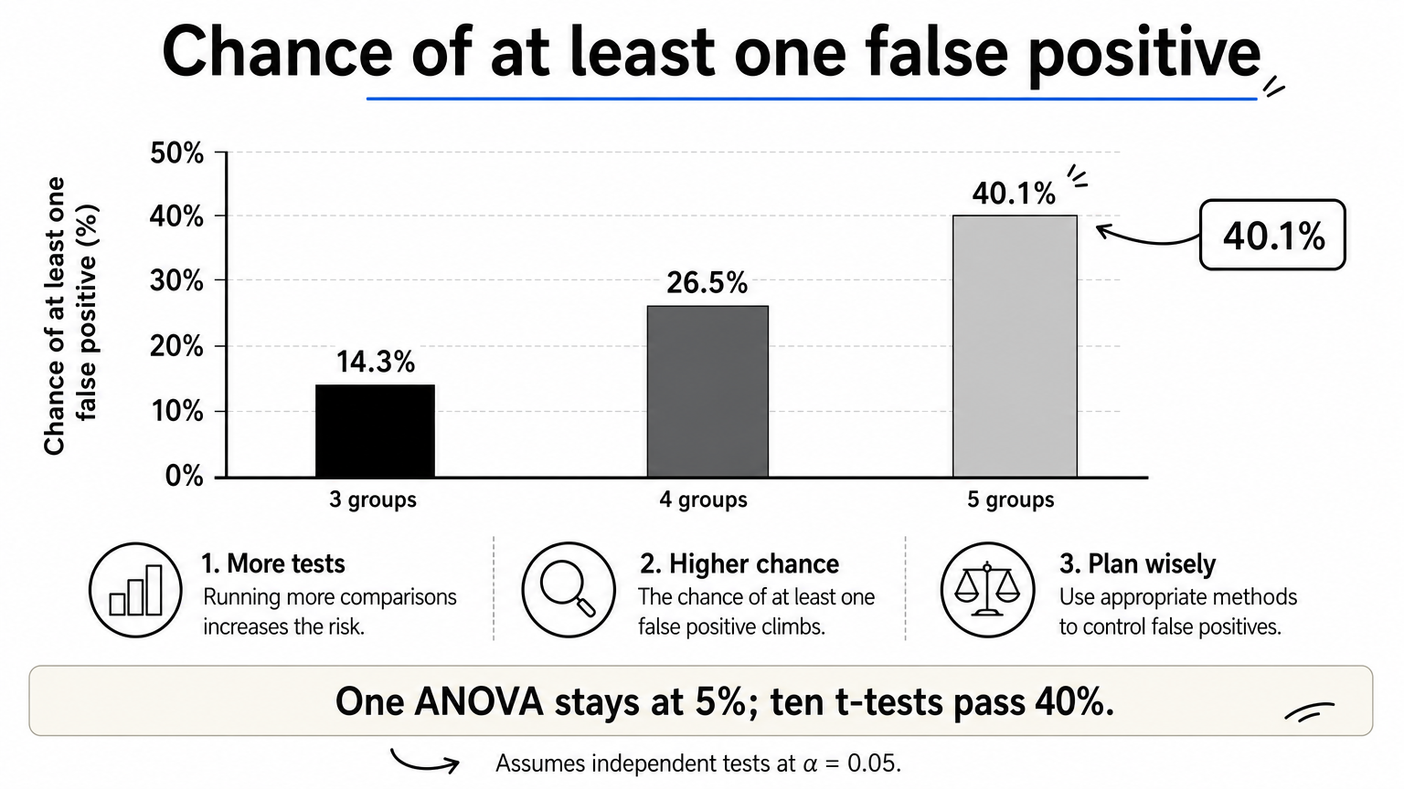
A t-test compares two means. With three groups you would need three t-tests, and each one carries a 5% false-positive risk at α = 0.05. Those risks accumulate. The table shows the approximate chance of at least one false positive, assuming independent tests.
| Number of groups | Pairwise t-tests needed | Chance of at least one false positive |
|---|---|---|
| 3 | 3 | 14.3% |
| 4 | 6 | 26.5% |
| 5 | 10 | 40.1% |
ANOVA runs a single test at your chosen α, so the error rate stays at 5%. With exactly two groups, ANOVA and the pooled two-sample t-test give the same p-value, because F equals t squared.
One ANOVA keeps your false-positive rate at 5%, where ten t-tests would push it past 40%.
How to run an ANOVA test step by step
To run an ANOVA test, state your hypotheses, check three assumptions, run the test in software, and follow a significant result with a post hoc comparison. Here is the process for a one-way design, meaning one factor with several levels.
Check the assumptions first
Before you trust the p-value, confirm that your data fit the test:

- Independence: each observation belongs to one group and does not depend on another. Repeated measures on the same people need a repeated-measures ANOVA instead.
- Approximate normality: residuals within each group should look roughly normal. Check a Q-Q plot or run a Shapiro-Wilk test.
- Equal variances: group spreads should be similar. Levene's test checks this.
The steps
- Write the hypotheses: H0 says μ1 = μ2 = μ3, and H1 says at least one mean differs.
- Choose α, usually 0.05.
- Arrange the data in two columns: the outcome and the group label.
- Check the assumptions above.
- Run the test and record F, both degrees of freedom, and the p-value.
- If p is below α, run a post hoc test and report an effect size.
Where to run it
You can run an ANOVA test in most statistical tools. Yes, Excel works too: enable the Analysis ToolPak, then use the single-factor option.
| Tool | How to run a one-way ANOVA |
|---|---|
| Excel | Data > Data Analysis > Anova: Single Factor |
| SPSS | Analyze > Compare Means > One-Way ANOVA |
| R | summary(aov(outcome ~ group, data = df)) |
| Python | scipy.stats.f_oneway(a, b, c) |
If you would rather describe the comparison in plain English, PlotStudio AI runs the test on your machine from an uploaded CSV. Verification Mode lets you review and edit the plan, including methods and assumptions, before anything executes. You can then export the code as a Jupyter notebook. The choice of test and the interpretation stay with you.
Check independence, normality and equal variances before you read the p-value, because the p-value is only as good as those assumptions.
How the F statistic is calculated
The ANOVA test statistic is F, the ratio of between-group variance to within-group variance. A ratio near 1 means the groups look alike. A ratio well above 1 means the group means are spread out more than the noise inside the groups explains.
The logic behind F
F equals MSB divided by MSW. MSB is the mean square between groups: the sum of squares between groups divided by k − 1, where k is the number of groups. MSW is the mean square within groups: the sum of squares within groups divided by N − k, where N is the total sample size.
People often ask whether ANOVA is just an F test. Almost. ANOVA is an F test applied to partitioned variance. Other procedures also use F, such as comparing two variances, so "F test" is the broader label.
A worked example with three groups
Imagine recovery scores for three treatments, three patients each. The numbers are made up to keep the arithmetic visible. Group A scored 4, 5, 6 (mean 5), group B scored 6, 7, 8 (mean 7), and group C scored 8, 9, 10 (mean 9). The grand mean is 7.

| Quantity | Calculation | Value |
|---|---|---|
| Sum of squares between | 3(5−7)² + 3(7−7)² + 3(9−7)² | 24 |
| Sum of squares within | 2 + 2 + 2 | 6 |
| Degrees of freedom | k − 1 = 2 and N − k = 6 | 2, 6 |
| MSB and MSW | 24 / 2 and 6 / 6 | 12 and 1 |
| F | 12 / 1 | 12 |
| p-value | F(2, 6) = 12 | 0.008 |
The critical F at α = 0.05 with 2 and 6 degrees of freedom is about 5.14. Our F of 12 is far beyond it, so you reject the null.
F is simply the signal between your groups divided by the noise within them.
Reading and reporting your ANOVA results
A significant ANOVA result means the group means are not all equal, so your next job is to find where the difference lies and how large it is. Report F, both degrees of freedom, the p-value, and an effect size.
Interpreting the p-value and effect size
For the example above, you would write: F(2, 6) = 12.00, p = .008, η² = .80. Eta squared is the sum of squares between divided by the total, here 24 / 30. Common rules of thumb call about 0.01 small, 0.06 medium, and 0.14 large. A p-value alone says nothing about practical importance, so always report the effect size too.
Post hoc tests and when assumptions fail
Run Tukey HSD to find which pairs differ. In our example the critical studentized range is about 4.34, so the honestly significant difference is 4.34 × √(1/3), roughly 2.51. Groups A and C differ by 4, which exceeds it. A versus B and B versus C differ by 2 each, which does not. So only the extreme pair is distinguishable at this sample size.
If variances are unequal, use Welch's ANOVA. If small samples are clearly non-normal, the Kruskal-Wallis test is the nonparametric alternative.
One-way versus two-way ANOVA
A one-way ANOVA test handles one factor, such as treatment. A two-way ANOVA handles two factors, such as treatment and sex, and also tests whether the factors interact. Choose by counting the grouping variables in your design.
A significant ANOVA only opens the question, because the post hoc test and effect size tell you where the difference is and whether it matters.
Putting the ANOVA test to work
An ANOVA test compares three or more group means in one step, keeps your false-positive rate at your chosen α, and reports its result as an F statistic built from between-group and within-group variance. Check the assumptions, run the test, then use Tukey HSD and an effect size to say which groups differ and by how much.
The calculation is the easy part. The judgment about design, assumptions and interpretation is yours. If you want software to handle the code while you keep control of the method, you can try PlotStudio AI free on your own dataset and review every step before it runs.