Can your forecasting tool explain what happened to missing observations, or does it return a convincing chart? Time series analysis software should fit models, diagnose errors, quantify uncertainty, and preserve a reproducible record. For research data analysis, PlotStudio AI adds an agentic workflow, while Python, R, SAS, and Excel offer different balances of control, scale, and accessibility.
Time Series Analysis Software Options Compared
Time series analysis software estimates, forecasts, and checks models for data indexed by time. A useful workflow includes model fitting, residual diagnostics, prediction intervals, anomaly flags, and exportable results.
| Option | Category | Model coverage | Reproducibility | Best fit |
|---|---|---|---|---|
| PlotStudio AI | Agentic analytics desktop app | ARIMA, SARIMAX, and GARCH through generated Python | Code shown for each step; Jupyter and PDF export | Researchers who need an investigation with an audit trail |
| statsmodels | Python library | AR, VAR, ARMA, and state-space models with Kalman filtering | Scripted workflows and saved results objects | Analysts already working in Python |
| R stats, forecast, and feasts | R packages | arima(), StructTS(), exponential smoothing, and STL-style decomposition |
Scripted, versionable workflows | Statisticians and econometricians |
| SAS Forecast Server | Commercial forecasting suite | Automatic model selection, hierarchical forecasting, and BY-group processing | Procedure-based workflows managed within SAS | Organizations forecasting many related series |
| Excel | Spreadsheet | Exponential smoothing through FORECAST.ETS |
Formula-based records requiring manual discipline | Quick forecasts for a small collection of series |
What each option asks of the analyst
PlotStudio AI can be considered a Julius AI alternative for researchers who need multi-step analysis, local Python execution, and a reproducible investigation record. The convenience doesn't remove the need to inspect the proposed method and validate its outputs.
statsmodels suits researchers who want direct access to estimation settings and fitted results. You supply the surrounding workflow, including data checks, backtesting, and reporting.
R suits teams that already organize statistical work in scripts and packages. Its flexibility comes with responsibility for package compatibility, data structures, and a consistent project environment.
SAS Forecast Server targets organizational forecasting rather than isolated notebook experiments. The SAS forecasting history documents its support for automatic model generation, hierarchical forecasting, and BY-group processing. For related series, test the reconciliation workflow as well as the individual forecasts.
Excel is approachable when the forecast is a small part of an existing workbook. However, a formula doesn't automatically document transformations, validation cutoffs, or why an analyst excluded an observation.
Selection rule: Match the tool to your number of series, coding skill, and data sensitivity, not the length of its algorithm menu.
These options fall into code libraries, commercial suites, and spreadsheet or agentic interfaces. Researchers combining forecasting with causal or panel analysis should also consider how their econometrics software fits the wider project. A forecasting tool shouldn't force the team to rebuild its entire research workflow.
Model Families and What Each One Handles
Start with the structure of the observations, not the model you've heard mentioned most often. A single demand series, a collection of regional indicators, and irregular clinical measurements present different estimation problems.
ARIMA is a reasonable candidate when a single regularly spaced series retains autocorrelation after appropriate differencing. For weekly demand, differencing may remove a changing level, leaving a process whose remaining dependence can be modeled with autoregressive and moving-average terms.
| Model family | Handles | Typical data | Watch for |
|---|---|---|---|
| ARIMA(p,d,q) | Autocorrelation remaining after differencing | A single series made roughly stationary | Residual autocorrelation and over-differencing |
| SARIMAX | Seasonal terms plus exogenous regressors | Monthly sales with price or holiday drivers | Future regressor values must be available at forecast time |
| GARCH(p,q) | Time-varying conditional variance | Daily financial returns | Models volatility, not the series level |
| ETS | Level, trend, and seasonality | Demand with reasonably stable patterns | Limited direct handling of external drivers |
| State-space with Kalman filtering | Missing observations and latent components | Sensor or clinical series with gaps | Sensitive specification and potentially demanding estimation |
| Forecast-residual anomaly detection | Observations outside prediction intervals | Operational metrics and monitoring | Thresholds depend on interval calibration |
Match the model to the question
SARIMAX adds seasonal structure and external predictors. For monthly sales, a planned price change can be useful; a future realized economic indicator isn't available unless you're explicitly forecasting it or constructing scenarios.
ETS, or exponential smoothing, provides a useful competing explanation based on level, trend, and seasonality. It isn't assumption-free: the selected error, trend, and seasonal forms still need to suit the observations.
GARCH answers a different question. When financial returns alternate between calm and turbulent periods, the target may be conditional variance rather than expected demand or price. Our financial methods include GARCH volatility models, RSI and MACD momentum indicators, and Bollinger Bands. Indicators summarize behavior; they aren't interchangeable with a probabilistic forecasting model.
State-space models describe observed measurements through an underlying, potentially unobserved process. For clinical data, distinguish scheduled measurements that are missing from irregular visit times before choosing that representation.
The CRAN forecastsuite documentation lists ARIMA, seasonal ARIMA, ETS, grouped-series reconciliation, ensembles, rolling-origin validation, and residual diagnostics. That breadth illustrates why one family rarely suits every series.
An observation outside a prediction interval is a candidate anomaly, not proof of a faulty sensor or a scientific event. Investigate its context before deleting it. Use a time-series methods guide to establish plausible candidates, then fit contrasting families and compare residual behavior before committing.
Selection Criteria Analysts Should Test
A feature list describes what a vendor intends to support. An acceptance test establishes what your actual workflow can do.
Test the workflow rather than the menu
- Scalability: Run a representative workload with realistic series lengths and grouping levels. Check runtime, memory use, failed fits, and whether totals remain consistent with their component forecasts.
- Reproducibility: Restart the environment and rerun the analysis. Preserve package versions, fitted parameters, data snapshots, and random seeds wherever the procedure uses randomness.
- Model coverage: Fit the required seasonal terms, external regressors, volatility models, or latent components. A model name in a menu doesn't establish that the implementation supports your specification.
- Verifiability: Inspect transformation code, convergence messages, residual checks, and prediction intervals. Require an explicit missing-data policy rather than accepting an unexplained reduction in row count.
- Privacy: Trace both computation and information transfer. Local execution and external AI requests are separate parts of the workflow, so institutional approval must consider both.
The statsmodels time-series documentation describes classical models alongside state-space infrastructure for maximum-likelihood estimation, Kalman filtering and smoothing, forecasting, and diagnostics. That infrastructure matters because supported state-space formulations can accommodate missing observations during estimation instead of requiring blanket deletion or preliminary imputation.
An acceptance test for missing observations
Take a representative series containing internal gaps and fit an ARIMA or SARIMAX specification using a missing-observation-capable implementation. Confirm that the time index remains intact, estimation completes, and the software has not compressed the gaps into adjacent observations.
Inspect convergence, fitted parameters, residual autocorrelation, and checks for changing variance. Then compare its forecasts and intervals with a separate workflow that imputes the gaps first, documenting the imputation method.
Don't assume that either result is automatically correct. Large differences identify a sensitivity worth investigating, especially if gaps occur during unusual operating conditions.
Missing values on a regular calendar and irregularly spaced measurements aren't the same problem. Preserving timestamps is necessary, but it doesn't by itself make a discrete-time model suitable for arbitrary observation intervals.
The Physiome-ODE benchmark presented at ICLR introduced 50 biologically derived datasets and found substantial changes in model rankings relative to conventional evaluation datasets. For researchers, the practical implication is to examine sampling-gap distributions, entity-specific observation patterns, and why measurements occurred.
A larger model isn't automatically a better model. Your forecasting accuracy assessment should make it possible to separate an unsuitable method from an unsuitable observation process, rather than treating both as an algorithm-selection problem.
How to Build and Validate a Forecast Without Leakage
Consider a hypothetical dataset containing 120 months of regional electricity demand. The planning task requires a three-month operational horizon, and the candidates are SARIMAX and ETS.
The forecast accuracy chapter in Forecasting: Principles and Practice describes reserving roughly 20% of observations as a common starting point, while emphasizing that the appropriate test size depends on the available sample and forecast horizon. In this hypothetical example, that would leave approximately 24 months for evaluation, enough to examine successive forecasting origins rather than only a final forecast.
The visual summarizes the forecasting task; its final validation segment is a single operational horizon, not a replacement for the longer backtest.
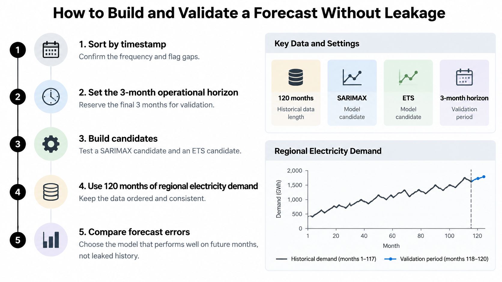
A chronological forecasting protocol
Sort and inspect the timestamps. Confirm monthly spacing, identify duplicate records, and flag missing months before fitting because an incorrectly constructed calendar changes the meaning of every lag. Keep missing demand distinct from demand recorded as zero.
Define the evaluation period and decision horizon. Use the hypothetical final test period for chronological evaluation, with each forecast predicting the next three months. Keep a final untouched assessment segment if you repeatedly adjust the workflow after reviewing backtest results.
Fit preprocessing within the training window. Learn scaling parameters, imputation rules, and differencing decisions using only observations available at that origin. Interpolating a training gap using a later test observation would leak information even if the model itself never reads the test table.
Generate rolling-origin forecasts. At each origin, fit or update the candidate using only preceding observations, then predict the next one, two, and three months. Choose an expanding window when older history remains relevant, or a fixed rolling window when the operational design deliberately excludes older regimes.
Calculate RMSE separately by horizon. Average squared forecast errors within each horizon and take the square root, so errors remain in the demand unit. This prevents strong near-term performance from concealing poor performance at the planning horizon.
Compare candidates on identical origins. Evaluate SARIMAX and ETS against the same observations and information set. Prefer the lower rolling-origin RMSE for the operational objective, rather than selecting whichever model fits historical observations most closely.
Inspect residuals and interval behavior. Check autocorrelation, changing variance, convergence problems, and whether intervals are plausibly calibrated. A flexible model can fit historical noise while producing worse future forecasts, so historical fit alone isn't an acceptance criterion.
Save the evaluation record. Store cutoff dates, training-window rules, feature availability assumptions, metric values, and the final specification together. A reviewer should be able to identify exactly what the analyst knew when each forecast was generated.
Make external predictors historically honest
Electricity demand may respond to weather, but realized future temperature isn't a legitimate input to a historical forecast. Use archived weather forecasts when available, or label weather scenarios explicitly and explain that their uncertainty may not be included in the demand interval.
The distinction between model selection and final testing is central to understanding cross-validation. Repeatedly examining a holdout and modifying the model turns that holdout into part of development.
Our application produces a permanent Analysis Page for every question, containing tables, charts, statistical tests, and interpretation in one structured document. For forecasting, include the evaluation protocol and assumptions in that saved record, not just the winning chart.
Automation Versus Manual Control in Practice
Automation is useful when the repeated work is well specified. Generating comparable diagnostic plots, fitting baseline candidates, and assembling results across related series can consume time without requiring a new scientific decision at every iteration.
The case for automation is straightforward: faster first drafts, consistent diagnostics, and less boilerplate code. The cost appears when automatic selection conceals consequential choices about transformations, differencing, outliers, or the evaluation window.
This comparison separates mechanical efficiency from analytical responsibility.
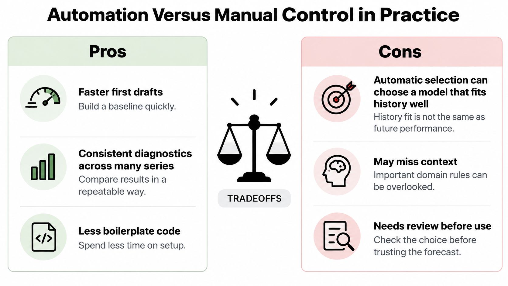
What an agent should do and what you should decide
Agentic analytics is data analysis performed by AI agents that can plan an investigation, execute analytical steps with real tools and code, inspect intermediate results, revise the approach, validate outputs, and synthesize a complete analysis.
That definition describes a workflow, not a guarantee of correctness. The analyst still needs to decide what outcome matters, what information would be available, and which assumptions are scientifically defensible.
An answer is an output; an analysis is an investigation. A forecast becomes useful when its assumptions, checks, and limitations are visible alongside its predicted values.
Our application runs analysis on the user's machine rather than on our servers. It provides generated code and a textual description of each analytical step, while Plan Mode lets users review, edit, and approve the proposed approach before execution.
For a clinical series, an analyst might reject routine interpolation because missed visits could reflect deteriorating health. For agricultural measurements, the analyst might retain an apparent outlier because it corresponds to a documented heat event. Neither decision should be delegated merely because software can execute it.
Where manual work still earns its cost
Manual scripting gives researchers precise control over unusual likelihoods, custom observation processes, and specialized sensitivity analyses. It also makes repetitive mistakes possible, such as applying a transformation to the complete dataset before constructing evaluation windows.
The useful middle path is to automate repeatable operations while requiring review at methodological decision points. Inspect the initial plan, examine intermediate data, and stop when the executed procedure no longer matches the scientific question.
The TSFM-Bench paper standardizes splitting, loading, normalization, and sampling across forecasting scenarios. Its emphasis is instructive: comparison procedures need as much attention as model execution.
Automation doesn't replace domain judgment, and a successfully executed script isn't evidence that the forecast is valid. Accept automated work only when its evaluation record supports the intended use.
Integrations and Export Formats for Research Teams
Start with an unambiguous input table. A CSV or Excel file can contain a consistently formatted timestamp column and a value column for each series; for many entities, a long table with timestamp, entity identifier, and measurement may be easier to manage.
Record units, timezone where relevant, and whether timestamps describe measurement time or reporting time. Preserve raw observations separately from cleaned and aggregated tables so collaborators can reconstruct the preparation process.
Connect the statistical environment to the data
The CRAN Econometrics task view describes base R's ts class for regularly spaced observations, alongside ar(), arima(), and StructTS(). Its surrounding ecosystem includes financial time-series structures, decomposition and feature extraction through feasts, and connections to X-13ARIMA-SEATS, the U.S. Census Bureau's seasonal-adjustment program.
These are complementary components, not interchangeable file formats. A regular time-series object encodes a sampling structure; converting an irregular clinical table into that object requires an explicit modeling decision.
For Python teams, pandas can manage timestamps, joins, and reshaping, while statsmodels supplies estimation. Keep preparation and estimation in the same runnable pipeline rather than exporting an undocumented intermediate spreadsheet.
Teams joining external predictors should preserve release timing as well as observation dates. A revised economic series may contain values that weren't available when the original forecasting decision occurred.
Export an analysis that another researcher can use
Our Jupyter export bundles code, data, and plots for rerunning the analysis. A PDF provides a read-only record for supervisors, collaborators, or manuscript review, but it doesn't replace executable code and the required environment.
A practical handoff checklist is:
- Timestamp contract: Document date format, frequency, timezone, duplicate handling, and the meaning of missing rows.
- Evaluation record: Store training cutoffs, forecast targets, predictor availability, and window settings.
- Executable package: Include the notebook, permitted data, package requirements, and any external input dependencies.
- Manuscript record: Keep the PDF with the matching manuscript version and identify exploratory versus confirmatory results.
For sensitive datasets, reproducibility may require controlled access rather than distributing raw participant records. The objective is an authorized collaborator's ability to reconstruct the analysis, not unrestricted sharing.
Good data integration practices preserve provenance through every conversion. A polished report with an untraceable input table isn't a complete research handoff.
Choose the Setup for Your Next Forecast
Pick the setup that makes your most consequential error easiest to catch. A student needs to see how a transformation changes the series. An operations team needs a failed forecast to surface before it drives a staffing decision. The right choice is the workflow that exposes gaps, leakage, and audit trails while you can still act.
A small first project makes those checks concrete. One series with a known history and a decision you can describe in a sentence will teach you more than a sprawling trial on every model family.
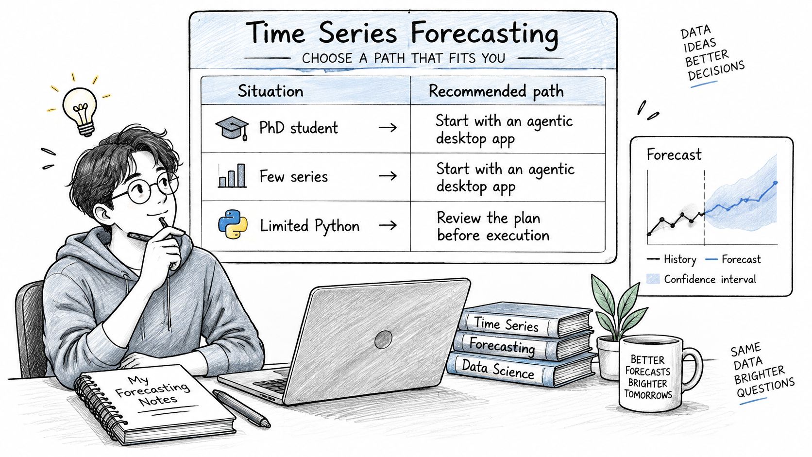
| Your situation | Starting setup | Acceptance requirement |
|---|---|---|
| PhD student with limited Python experience | Agentic desktop analysis with plan review and visible code | Can explain each transformation and rerun the method from generated code |
| Data scientist managing related series | Scripted statsmodels or R evaluation, with agentic exploration for side checks | Comparable forecast origins, explicit failure logs, and grouping that respects shared drivers |
| Product manager needing monitored forecasts | Forecasting workflow connected to monitoring | Documented anomaly thresholds and a named owner for validation |
| Researcher handling sensitive records | Institution-approved computation and model connection | Verified permissions for any data sent to an external model |
If you choose an agentic workflow, ask for the permanent analysis page. It should collect the tables, charts, tests, interpretation, and generated code in one document, so a collaborator can review the transformation history later.
PlotStudio AI runs as a desktop application on Mac and Windows. The BYOK subscription lets you connect the AI provider your institution already funds, subject to its policies. Analysis runs on your machine, so the data stays local. Local computation alone does not authorize sending sensitive records through an external model connection. Treat compute location and model endpoint as separate permissions.
A live demo can shorten the learning curve: bring a CSV, ask a question, and watch how the system parses dates, flags missing values, and records each step before you commit.
Frequently asked questions
What is the best time series analysis software for researchers?
Choose statsmodels or R for direct statistical programming, SAS for organized large-scale forecasting, or an agentic desktop workflow for guided investigation. The best fit is the one your team can validate and maintain.
Can time series software analyze irregular clinical measurements?
Sometimes, but support for missing observations does not establish support for irregular timing. Check whether the method represents elapsed time and the visit process appropriately.
Can AI write the forecasting methods section?
It can draft a description from saved code and outputs. The researcher must verify that the description matches the executed procedure and does not convert exploratory findings into confirmatory claims.
Download and try PlotStudio AI with one series you already know well. Inspect whether its preparation, forecast, and uncertainty match your expectations. If the output cannot show what changed, how missing rows were handled, and which cutoffs were used, keep looking. The free trial is there for that test.