A p-value in hypothesis testing is the probability of getting results at least as extreme as yours if the null hypothesis were true. When the p-value is at or below your significance level, usually 0.05, your data are hard to explain by chance alone, so you reject the null hypothesis. When it is above that level, your data are consistent with random variation, so you do not reject it. The p-value measures surprise. It does not tell you the probability that your hypothesis is right.
This article explains why the p-value matters, how to calculate it step by step, and how it plays out in a full worked example. You will also see how to read values like 0.05 and 0.001, and which common misreadings to avoid. If you have ever copied a p-value from software into a manuscript without being sure what it said, this is for you.
We build PlotStudio AI, a desktop workspace where researchers run statistical tests and see the test statistic, the p-value, and the Python code behind them. The software produces the number quickly. Deciding what it means for your study still takes your judgment, and that is the skill this guide covers.
Why the p-value matters in hypothesis testing
The p-value gives you one standardized way to decide whether an observed difference is big enough to take seriously or small enough to be sampling noise. Without it, "these groups look different" is an opinion. With it, you can state how surprising the gap would be if nothing real were going on.
The problem it solves
Samples vary. If you measure two groups of 15 people, their averages will differ even when the treatment does nothing. The question is never whether a difference exists in your sample. It is whether the difference is larger than chance alone would typically produce.

The p-value answers that by assuming no real effect and asking how often a result this extreme would still appear. A p-value of 0.03 means that under the null hypothesis, roughly 3 in 100 samples would show a result at least this extreme. That is the logic behind statistical significance, and every reported "significant" finding rests on it.
How it connects to the null hypothesis and alpha
Every test starts with two competing statements. The null hypothesis (H0) says there is no effect, difference, or relationship. The alternative hypothesis (H1) says there is. You choose a significance level, alpha (α), before you look at the data. Alpha is the false-positive risk you accept, or the chance of rejecting a true null hypothesis (a Type I error).
The decision rule is short: if p ≤ α, reject H0. If p > α, fail to reject H0. Here is how the pieces fit together.
| Term | What it means | Typical value |
|---|---|---|
| Null hypothesis (H0) | No effect or no difference | Fixed by your question |
| Alternative hypothesis (H1) | An effect or difference exists | One-tailed or two-tailed |
| Significance level (α) | Type I error rate you accept | 0.05, sometimes 0.01 or 0.10 |
| Test statistic | How far your data sit from H0 | t, z, chi-square, or F |
| P-value | Probability of a result this extreme if H0 is true | Between 0 and 1 |
The p-value tells you how well your data fit a world where nothing is happening.
How to calculate a p-value step by step
You calculate a p-value by turning your data into a test statistic, then finding the area in the tail of that statistic's distribution under the null hypothesis. Software does the lookup for you, but knowing the steps tells you what the output means.
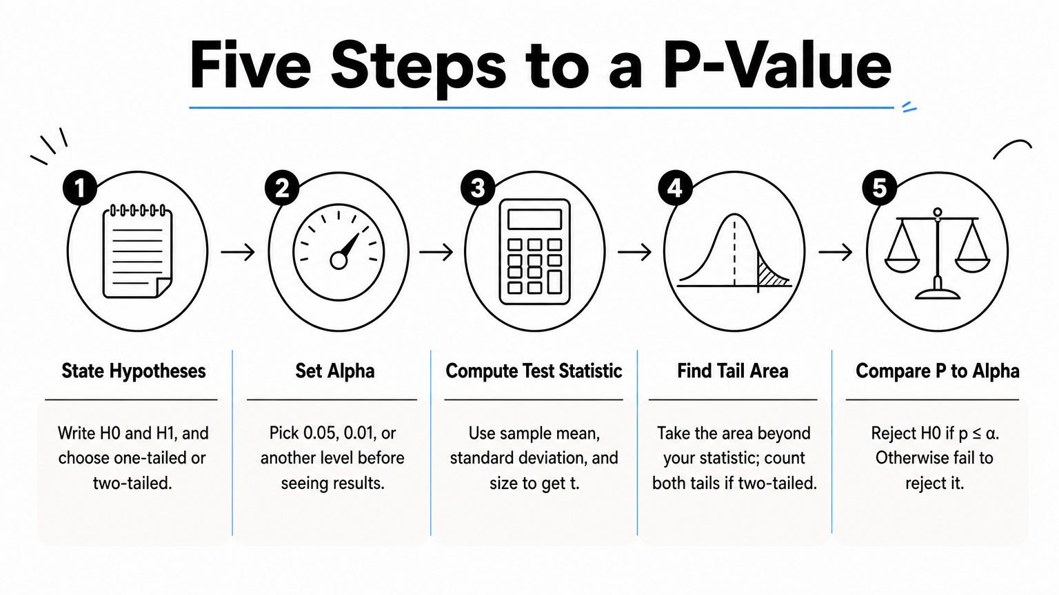
The five steps
- State the hypotheses. Write H0 and H1, and decide whether the test is one-tailed or two-tailed.
- Set alpha. Pick 0.05, 0.01, or another level before seeing results.
- Compute the test statistic. Use your sample mean, standard deviation, and size, for example t = (x̄ − μ0) / (s / √n).
- Find the tail area. Using the distribution that applies when H0 is true, take the area beyond your statistic. For a two-tailed test, count both tails.
- Compare p to alpha. Reject H0 if p ≤ α. Otherwise fail to reject it.
A two-tailed p-value is exactly twice the one-tailed value when the distribution is symmetric, as with the t and normal distributions. Choose the direction of your test before the analysis, not after you see which way the data lean.
Which test produces the p-value
The test you choose determines the test statistic and the distribution used for the p-value.
| Test | Use it when | Reference distribution |
|---|---|---|
| z-test | Large sample or known population variance | Standard normal |
| t-test | Comparing means with unknown variance | t, with degrees of freedom |
| Chi-square test | Comparing categorical counts | Chi-square |
| F-test or ANOVA | Comparing three or more group means or variances | F |
| Correlation test | Checking a linear relationship | t, based on r |
Picking the wrong test gives a p-value that looks fine and means nothing, because each test assumes things about your data, such as normality or independence. When you run analyses in PlotStudio AI, Verification Mode lets you review the proposed method and its assumptions before anything executes, and you can read the generated code afterward.
A p-value is only as trustworthy as the test behind it, so check the assumptions first.
Worked example: a one-sample t-test
In this example you test whether a treatment changes systolic blood pressure, using a one-sample t-test on hypothetical data. The numbers are invented to show the mechanics, not taken from a real trial.
The setup
Fifteen patients each have their blood pressure change recorded after eight weeks. The mean change is a 5.0 mmHg reduction, and the standard deviation is 7.75. You want to know whether that average differs from zero.

- H0: the true mean change is 0.
- H1: the true mean change is not 0 (two-tailed).
- α = 0.05.
The calculation and decision
Start with the standard error: 7.75 / √15 ≈ 2.0. The test statistic is t = 5.0 / 2.0 = 2.5, with n − 1 = 14 degrees of freedom. The area in the right tail beyond t = 2.5 is about 0.0127. Because the test is two-tailed, you double it to get p ≈ 0.0254. You can check this in Python:
from scipy import stats

t_stat = 2.5
df = 14
p_value = 2 * stats.t.sf(abs(t_stat), df)
print(round(p_value, 4))  # 0.0254
In Excel, the equivalent is =T.DIST.2T(2.5, 14). Since 0.0254 is below 0.05, you reject the null hypothesis and conclude the mean change differs from zero. That conclusion depends on the alpha you set, as this table shows.
| Alpha | p = 0.0254 compared to alpha | Decision |
|---|---|---|
| 0.10 | Smaller | Reject H0 |
| 0.05 | Smaller | Reject H0 |
| 0.01 | Larger | Fail to reject H0 |
If you had committed in advance to a one-tailed test for a reduction, the p-value would be 0.0127, and you would still fail to reject at α = 0.01. The data did not change. Only your threshold did, which is why you fix alpha first.
The same p-value can lead to different decisions depending on the alpha you chose beforehand.
How to interpret p-values without misreading them
To interpret a p-value, compare it to your alpha for the decision, then judge the size of the effect for the meaning. A p-value answers whether a result is surprising under the null. It does not say whether the result is large or important.
What 0.05, 0.001, and values above 0.05 tell you
A p-value of 0.05 sits exactly on the conventional line. By the standard rule (p ≤ α), it counts as significant at α = 0.05, but it is borderline evidence at best. The 0.05 cutoff is a convention, not a law of nature. A p-value of 0.001 is statistically significant at all the usual levels, and it means the data would be very rare under the null.
| P-value | Common reading | Caution |
|---|---|---|
| ≤ 0.001 | Very strong evidence against H0 | Can still be a tiny effect |
| 0.001 to 0.01 | Strong evidence against H0 | Check effect size |
| 0.01 to 0.05 | Moderate evidence against H0 | Sensitive to the test chosen |
| 0.05 to 0.10 | Weak or suggestive evidence | Not significant at 0.05 |
| > 0.10 | Little evidence against H0 | Not proof of no effect |
These labels are rules of thumb, and fields differ in what they expect. When your p-value is greater than 0.05, you fail to reject the null. You have not shown that the null is true, only that your data did not give enough evidence against it. A small sample can easily produce that outcome even when a real effect exists.
Four misreadings to avoid
- It is not the probability that H0 is true. It is calculated by assuming H0 is true.
- It is not the probability that chance caused your result. Chance is built into the calculation, so the number cannot also measure it.
- It is not an effect size. With a large enough sample, a trivial difference produces a tiny p-value. Report the effect size and a confidence interval next to it.
- It is not a license to run many tests. At α = 0.05, 20 independent tests on pure noise have about a 64% chance of producing at least one "significant" result. Plan your comparisons, and use a correction such as Bonferroni when you run several.
A small p-value says your data are surprising under the null, not that your finding is large or true.
Using p-values with confidence
The p-value tells you how surprising your data are if the null hypothesis holds. You set alpha first, pick a test that fits your data, compute the statistic, and compare p to alpha. Then you read the result alongside the effect size and confidence interval instead of treating 0.05 as a pass-or-fail line.
If you want to practice on your own data, try PlotStudio AI free. You can run a test, check which method and assumptions it uses, and read the p-value together with the code that produced it.