ANOVA tests whether the means of three or more groups differ, and it makes that call with an F-test. The F-test divides the variance between your group means by the variance within your groups. The result is the F-statistic. A value near 1 means the groups look no more different than random noise would make them. A large value means the gaps between groups are too big to blame on chance. That is why the ANOVA and F test are always mentioned together: ANOVA is the method, and the F-test is the calculation that delivers its verdict.
This article explains why the F-test matters in ANOVA, how the F-statistic is calculated, and how to read it. You will follow one worked example from raw numbers to a finished ANOVA table. Then you will see how to read the F-value and p-value, which assumptions to check, and how to run and report the test.
PlotStudio AI runs ANOVA for researchers inside an analysis workspace, and the tables it produces report an F-value and a p-value. If you know what those two numbers mean, you can check the analysis instead of trusting it blindly.
Why the F-test sits at the heart of ANOVA
The F-test turns ANOVA's breakdown of variance into a decision about group means. ANOVA splits the total variability in your data into a part explained by group membership and a part left over as noise. The F-test compares the two and tells you whether the explained part is larger than chance would produce.
Are ANOVA and the F-test the same thing?
No. ANOVA is a method, and the F-test is the test it uses to reach a conclusion. In a one-way ANOVA the F-test is the only test in the table, so people treat the two terms as synonyms. The F-test is more general, though. It compares any two variance estimates, so it shows up in other places:
| Use of the F-test | What the ratio compares |
|---|---|
| One-way ANOVA | Variance between group means vs. variance within groups |
| Overall significance of a regression | Variance explained by the model vs. residual variance |
| Comparing two variances | Variance of one sample vs. variance of another |
| Comparing nested models | Improvement in fit per added term vs. residual variance |
The idea is the same each time. You form a ratio of two mean squares, and that ratio follows an F-distribution when the null hypothesis is true. Only the pair of variances changes.
Why you test means by comparing variances
Asking whether means differ is really asking whether the means vary. Group averages of 8.8, 8.9, 9.0 and 9.1 barely vary, so you would not call them different. Averages of 5, 7, 9 and 11 vary a lot. But "a lot" depends on noise. If individual observations scatter widely inside each group, a wide spread among group averages is easy to get by luck.

So ANOVA treats the spread among group means as the signal and the spread inside groups as the noise. The F-statistic is the signal-to-noise ratio.
ANOVA asks whether your group means vary more than the noise inside each group would allow.
Why not just run several t-tests?
Every extra test adds another chance of a false positive. With three groups you need three pairwise t-tests. At a 0.05 threshold each, the chance of at least one false positive is roughly 1 − 0.95³, or about 14%. With four groups (6 comparisons) it climbs to about 26%. With five groups (10 comparisons) it reaches about 40%.
The F-test avoids this. It asks one question, "are all the means equal?", and answers it with a single test at 0.05. If you then need to know which pairs differ, you use a post hoc procedure built to control the error rate, which comes up later in this article.
How the F-statistic is calculated, step by step
The F-statistic is the mean square between groups divided by the mean square within groups. Each mean square is a sum of squares divided by its degrees of freedom. Software does this instantly, but doing it once by hand shows you what the number means.
The formula and its parts
For k groups and N observations in total, follow these steps:
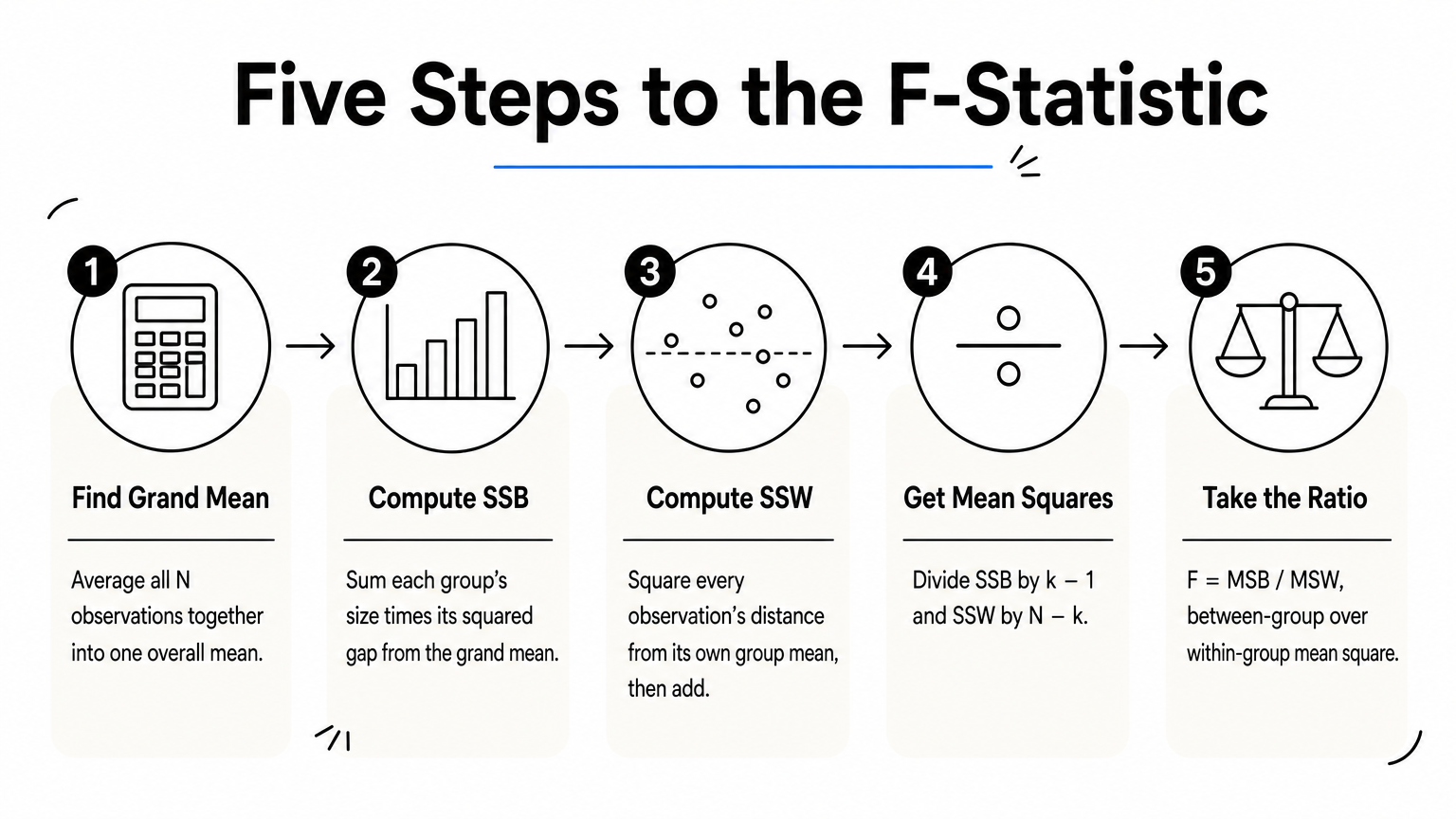
- Find the grand mean of all N observations.
- Compute the sum of squares between groups (SSB). For each group, take its size times the squared distance between the group mean and the grand mean, then add these up. Its degrees of freedom are k − 1.
- Compute the sum of squares within groups (SSW). For every observation, square its distance from its own group mean, then add everything up. Its degrees of freedom are N − k.
- Divide each sum of squares by its degrees of freedom to get MSB and MSW.
- Divide: F = MSB / MSW.
The division by degrees of freedom matters. A sum of squares grows as you add observations, so raw sums from different sources are not comparable. Mean squares put both on the same footing. If the null hypothesis is true, both estimate the same population variance, and F lands near 1.
A worked example with three groups
Suppose a small trial measures the reduction in systolic blood pressure (mmHg) in 15 patients, five per group. These numbers are invented for illustration.
| Group | Values | Mean |
|---|---|---|
| Placebo | 3, 5, 6, 5, 6 | 5 |
| Low dose | 5, 7, 8, 6, 9 | 7 |
| High dose | 7, 9, 10, 8, 11 | 9 |
The grand mean is (25 + 35 + 45) / 15 = 7. Between groups, SSB = 5(5 − 7)² + 5(7 − 7)² + 5(9 − 7)² = 20 + 0 + 20 = 40, with 3 − 1 = 2 degrees of freedom. Within groups, the squared distances from each group mean add up to 6 + 10 + 10 = 26, with 15 − 3 = 12 degrees of freedom.
That gives MSB = 40 / 2 = 20 and MSW = 26 / 12 ≈ 2.17. So F = 20 / 2.17 ≈ 9.23. The variation between group means is about nine times the variation within groups.
Reading the ANOVA table
Statistical software lays these results out in a standard table. Here is the same example:
| Source | SS | df | MS | F |
|---|---|---|---|---|
| Between groups | 40 | 2 | 20.00 | 9.23 |
| Within groups | 26 | 12 | 2.17 | |
| Total | 66 | 14 |
The sums of squares add up (40 + 26 = 66), and so do the degrees of freedom (2 + 12 = 14). If your output does not add up like this, something is wrong with the setup. With only two groups, the ANOVA F-test gives the same result as a two-sample t-test, and F equals t².
F is the mean square between groups divided by the mean square within groups, nothing more.
How to interpret the F-value and p-value
An F-value near 1 means your group differences are no bigger than noise, and larger values give stronger evidence against equal means. Whether a value is large enough depends on the degrees of freedom, so you judge it against a critical value or, more commonly, a p-value.
What the F-statistic tells you
F can never be negative, because it is a ratio of two variances. It is a unitless number, so on its own it does not describe how big the difference is in mmHg or any other unit. Instead it says how many times larger the between-group variance is than the within-group variance. In the example, 9.23 means the group means vary about nine times more than the noise would predict.
That is the answer to what the F in ANOVA tells you. It measures whether the differences among groups stand out above the background noise. It does not say which groups differ or by how much.
What counts as a good F-statistic
There is no universal cutoff. A "good" F is one that exceeds the critical value for your degrees of freedom at your chosen significance level. The critical value shrinks as the within-group degrees of freedom grow and as you add groups to the numerator. These are the critical values at α = 0.05:
| Numerator df | Denominator df | Critical F |
|---|---|---|
| 2 | 12 | 3.89 |
| 2 | 30 | 3.32 |
| 2 | 120 | 3.07 |
| 3 | 30 | 2.92 |
| 4 | 30 | 2.69 |
Our F of 9.23 with 2 and 12 degrees of freedom beats the critical value of 3.89. The matching p-value is about 0.004. That is the probability of getting an F at least this large if all three population means were equal. Because only large F-values count as evidence, the test is always right-tailed. A p-value below 0.05 lets you reject the null hypothesis that the group means are equal.
What a significant F does not tell you
A significant result says that at least one mean differs. It does not say which, and it does not say whether the difference matters in practice. For size, compute eta squared, which is SSB divided by the total sum of squares. In the example that is 40 / 66 ≈ 0.61, so group membership accounts for about 61% of the variability in blood pressure reduction.
With very large samples, tiny differences can produce a huge F and a minuscule p-value. Always report an effect size next to the F-test so readers can judge the practical weight of the finding.
A significant F says the means are not all equal. Effect size says whether the difference is worth caring about.
Assumptions to check and what to do after the test
The F-test in ANOVA is trustworthy when observations are independent, residuals are roughly normal, and group variances are similar. When they are not, you switch to an adjusted test. When F is significant, you follow up with a post hoc procedure.
The three assumptions to check
- Independence. Each observation must not influence another. Repeated measures on the same patient break this, and they need a repeated-measures ANOVA instead.
- Normal residuals. The errors within each group should be roughly bell-shaped. A Q-Q plot of residuals is the quickest check, and a Shapiro-Wilk test can back it up. The F-test tolerates mild departures, especially when groups are balanced and moderately sized.
- Equal variances. The spread within each group should be similar. Box plots show this at a glance, and Levene's test checks it formally. This one matters most when group sizes are unequal.

Independence is a design question, so you cannot fix it after the fact. The other two you can test and, if needed, work around.
What to do after the F-test
Your next move depends on what the checks and the F-value show:
| Situation | Next step |
|---|---|
| Significant F, variances similar | Tukey HSD to find which pairs differ |
| Significant F, variances unequal | Welch's ANOVA, then Games-Howell for pairs |
| Skewed data, small groups, or ordinal outcomes | Kruskal-Wallis test |
| Non-significant F | Stop. Report the effect size and confidence intervals |
Do not skip the post hoc step by running unadjusted t-tests after a significant F. That brings back the inflated false-positive rate you used ANOVA to avoid. Equally, do not go hunting for pairwise differences after a non-significant F.
Check the assumptions before you trust the F-value, and use a post hoc test, not repeated t-tests, to find which groups differ.
How to run and report the F-test in ANOVA
You can run a one-way ANOVA F-test in Python, R or Excel in a few lines or clicks, then report F with both degrees of freedom, the p-value and an effect size. Running the example from earlier is a good way to confirm you read the output correctly.
Running the test in code
In Python, SciPy's one-way ANOVA function takes one list per group:
from scipy import stats

placebo = [3, 5, 6, 5, 6]
low_dose = [5, 7, 8, 6, 9]
high_dose = [7, 9, 10, 8, 11]

f_stat, p_value = stats.f_oneway(placebo, low_dose, high_dose)
print(f_stat, p_value)
This prints an F of about 9.23 and a p-value of about 0.0037, matching the hand calculation. In R, summary(aov(reduction ~ group, data = df)) returns the full ANOVA table. In Excel, the Data Analysis ToolPak offers "Anova: Single Factor".
Reporting the result
Report the F-statistic with the between and within degrees of freedom in parentheses, then the p-value and effect size. Here is a sentence you can adapt:
A one-way ANOVA showed a significant effect of dose on blood pressure reduction, F(2, 12) = 9.23, p = .004, η² = .61.
Add the group means and standard deviations, the assumption checks you ran, and the post hoc results. Readers and reviewers expect all of that alongside the F-value.
If you would rather skip the code, PlotStudio AI lets you upload a dataset and ask for an ANOVA in plain English. In Verification Mode you can review the proposed plan, question it and edit the methods and assumptions before anything runs. You can also inspect the generated Python and export the result as a PDF report or Jupyter notebook. The judgment calls, such as whether the assumptions hold and what the result means for your study, stay with you.
Reading ANOVA results with confidence
ANOVA decides whether group means differ, and the F-test is its engine: a ratio of between-group variance to within-group variance. A value near 1 means noise. A value well above the critical value for your degrees of freedom means real differences. The p-value turns that into a probability, and eta squared tells you how much the groups matter.
Check independence, normality and equal variances first. If F is significant, find the differing pairs with a post hoc test. Report F with both degrees of freedom, the p-value and the effect size. Do the calculation by hand once, as in the example above, and the output of any software will make sense.
When you are ready to run an ANOVA on your own data, you can try PlotStudio AI on your own dataset. It is free to try, with no credit card required.