The Mann Whitney t test is the common search name for the Mann-Whitney U test, a rank-based method that compares two independent groups when a t-test would be risky. It is not actually a t-test. It is the nonparametric alternative to the independent samples t-test, and it asks whether values in one group tend to be higher than values in the other, not whether the two means differ. You may also see it called the Wilcoxon rank-sum test, which is the same test under another name.
That difference in question is why the test exists. Hospital stays, costs, biomarker concentrations, and 0 to 10 symptom scores are often skewed, bounded, or ordinal, and one extreme value can drag a mean far from where most of the data sit. Ranks keep only each value's position in the order, so the test stays stable where the t-test wobbles.
This guide covers why the test matters, how to run it by hand and in software on a worked example, how it differs from the t-test and Welch's t-test, when to choose it, and how to interpret and report the result. PlotStudio AI is built for researchers who run exactly these comparisons, so the workflow notes show how to check each decision yourself, whatever software you use.
Why the Mann-Whitney test matters when means mislead
The Mann-Whitney test matters because the t-test answers a question about means, and means are fragile when data are skewed, ordinal, or contaminated by outliers. When an average does not describe your outcome well, a test built on averages can mislead you in either direction.
Where the mean breaks down
Take length of stay after surgery. Most patients leave within a week, a few stay for a month, and one stays 38 days. That single patient lifts the group mean and inflates the standard deviation, and a t-test uses both to judge the gap between groups. The same thing happens with hospital costs, reaction times, viral loads, and enzyme levels. Skewed distributions and outliers distort both halves of the t statistic.

Ordinal data cause a different problem. A pain score of 8 is worse than 6, but nobody can say the scale is evenly spaced, so averaging assumes more than the scale promises. Ranking asks only which value is larger. That is why ordinal outcomes such as Likert items fit this test without any stretching.
Ranks fix both problems. You replace each value with its position in the pooled, sorted data. The 38-day stay gets the top rank whether it is 38 days or 380 days, so no single observation can pull the result very far.
What the test actually answers
The strict null hypothesis is that both groups come from the same distribution. The more useful reading is about probability: if you pick one observation at random from each group, the chance that group A's value is higher equals the chance that group B's value is higher, so both probabilities are 50%. Researchers call the departure from 50% the probability of superiority, and it is a natural effect size for this test.
Many textbooks say the test compares medians. That holds only when the two distributions have the same shape and differ by a shift. Medians are never used in the calculation, and two groups can share a median yet produce a significant result because their spread or skew differs. Medians are a valid summary only under the same-shape condition, so check the shapes before you word your conclusion.
The Mann-Whitney test compares ranks, not means, so it answers "do values in one group tend to be higher?" instead of "do the averages differ?"
What you give up
The trade is small. When data really are normal, the test has an asymptotic relative efficiency of about 0.95 against the t-test, meaning you need roughly 5% more observations to match its power. With heavy tails or outliers, the rank-based test can be the more powerful of the two.
The real limits are different. With only 3 observations per group, the smallest possible two-sided exact p-value is 0.10, so significance is out of reach no matter how clean the separation. With 4 per group the floor is about 0.029. You also lose a mean difference in original units, though the Hodges-Lehmann estimate, covered later, gives you a rank-based replacement.
How to run a Mann-Whitney test, step by step
You run the test by ranking all values together, summing the ranks for each group, converting a rank sum to U, and comparing U with a critical value or p-value. Software does the last step in one line, but doing a small example by hand shows you what the output means.
The steps by hand
Follow these six steps for two independent groups with sizes n1 and n2:
- State the hypotheses. The null is that values in neither group tend to be larger. The alternative, for a two-sided test, is that one group tends to be larger.
- Pool both groups and sort from smallest to largest.
- Assign ranks from 1 upward. Tied values share the average of the ranks they occupy.
- Add up the ranks for each group to get R1 and R2.
- Compute U1 = R1 − n1(n1 + 1)/2 and U2 = n1 × n2 − U1.
- Take the smaller of U1 and U2 as the test statistic and compare it with a critical value from a U table, or use the normal approximation.
Check your arithmetic with two identities. R1 + R2 must equal N(N + 1)/2 where N = n1 + n2, and U1 + U2 must equal n1 × n2.
A worked example with ties
These numbers are invented for illustration. A hospital compares length of stay in days under standard care (n = 6) and an enhanced recovery protocol (n = 6).
- Standard care: 7, 9, 12, 15, 21, 38
- Enhanced protocol: 3, 4, 5, 7, 8, 10
Pool the 12 values and rank them. The two 7s occupy ranks 4 and 5, so each gets 4.5.
| Days | Group | Rank |
|---|---|---|
| 3 | Enhanced | 1 |
| 4 | Enhanced | 2 |
| 5 | Enhanced | 3 |
| 7 | Standard | 4.5 |
| 7 | Enhanced | 4.5 |
| 8 | Enhanced | 6 |
| 9 | Standard | 7 |
| 10 | Enhanced | 8 |
| 12 | Standard | 9 |
| 15 | Standard | 10 |
| 21 | Standard | 11 |
| 38 | Standard | 12 |
The rank sums are R1 = 53.5 for standard care and R2 = 24.5 for the enhanced protocol. They add to 78, which equals 12 × 13 / 2, so the ranking is consistent. Then U1 = 53.5 − 21 = 32.5 and U2 = 36 − 32.5 = 3.5, and the smaller value, U = 3.5, is the test statistic.
For n1 = n2 = 6, the two-sided critical value at α = 0.05 is 5, and you reject the null when U is at or below it. Here 3.5 is below 5, so the result is significant. Because of the tie, software uses the normal approximation instead of the exact table. The mean of U under the null is 18, the tie-corrected standard deviation is about 6.23, and z is about −2.25 with a continuity correction, giving p of about 0.025.
Rank the pooled data, sum the ranks per group, convert to U, and let software handle the p-value.
Running it in software
In SPSS, choose Analyze, then Nonparametric Tests, then Legacy Dialogs, then 2 Independent Samples. Move your outcome into the test variable box, your grouping variable into the grouping box, define the two group codes, and keep the Mann-Whitney U box ticked. In Python and R, the same test is one call:
from scipy.stats import mannwhitneyu

standard = [7, 9, 12, 15, 21, 38]
enhanced = [3, 4, 5, 7, 8, 10]

result = mannwhitneyu(standard, enhanced, alternative="two-sided")
print(result.statistic, result.pvalue)
standard <- c(7, 9, 12, 15, 21, 38)
enhanced <- c(3, 4, 5, 7, 8, 10)

wilcox.test(standard, enhanced, conf.int = TRUE)
SciPy reports U for the first sample, so you get 32.5 here, and the smaller U is 36 − 32.5 = 3.5. R calls the statistic W but reports the same quantity, and it warns about ties because it cannot compute an exact p-value with them. Both give a p-value near 0.025.
If you would rather not write code, upload the CSV to PlotStudio AI and ask for the comparison in plain English. With Verification Mode on, you review the proposed plan and its assumptions before anything runs, so you can confirm it chose Mann-Whitney for the reasons you intended. You can also inspect the generated Python and export it as a Jupyter notebook, which makes the analysis easy to audit and reproduce.
Mann-Whitney vs t-test: how they differ
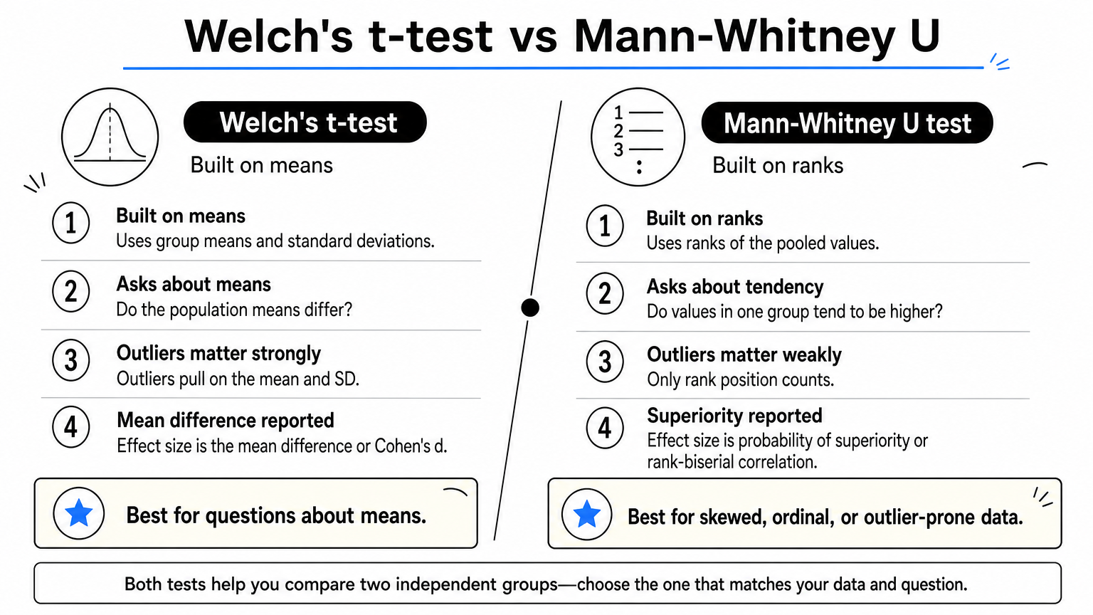
The t-test compares means using the raw values and relies on approximately normal sampling distributions, while the Mann-Whitney test compares ranks and needs no normality. Both handle two independent groups, so the choice comes down to your data type, your sample size, and the question you want to answer.
Side-by-side comparison
| Feature | Independent samples t-test (Welch) | Mann-Whitney U test |
|---|---|---|
| Built on | Group means and standard deviations | Ranks of the pooled values |
| Question answered | Do the population means differ? | Do values in one group tend to be higher? |
| Outcome type | Continuous | Ordinal or continuous |
| Normality | Needed for small samples, relaxed for large ones | Not required |
| Effect of outliers | Strong, through mean and SD | Weak, since only rank position counts |
| Same-shape condition | Not needed | Needed to describe results as a median difference |
| Typical effect size | Mean difference, Cohen's d | Probability of superiority, rank-biserial correlation |
| Power if data are normal | Highest | About 95% of the t-test's efficiency |
The label "Mann-Whitney t-test" is a misnomer worth correcting in your own writing. The statistic is U, not t, so report it as a Mann-Whitney U test.
Same data, different answers
Run Welch's t-test on the length-of-stay example and you get a different story. The group means are 17.0 and 6.2 days, t is about 2.27 with roughly 5.5 degrees of freedom, and p is about 0.07. The Mann-Whitney test gave p of about 0.025 on the same numbers.
The 38-day stay explains the gap. It pushes the standard care standard deviation to about 11.4 days against 2.6 for the enhanced group, and that inflated variance weakens the t statistic. The rank test only sees that all six standard care values sit mostly above the enhanced values. This is the situation behind the common forum question about one test being significant and the other not.
Do not treat that as permission to shop for the test that gives p below 0.05. Decide on the test before you look at the p-values, based on the outcome type, the shape of the data, and the question. Then report the one you planned.
Welch's t-test, Mann-Whitney, and the Wilcoxon name
Use Welch's t-test when your question is about means and your samples are moderate or large, since it handles unequal variances without an equal-variance assumption. Use Mann-Whitney when the outcome is ordinal, when samples are small and skewed, when outliers are real data you cannot remove, or when a rank-based question suits your research better. Welch's test is the sensible default over Student's pooled version for most work.
The Wilcoxon rank-sum test and the Mann-Whitney U test are the same test. Wilcoxon's W is the rank sum of one group, and U = W − n1(n1 + 1)/2, so the p-values match. Do not confuse either with the Wilcoxon signed-rank test, which is for paired data such as the same patients measured before and after treatment.
Choose between Welch and Mann-Whitney before you see the results, based on data type and the question, never on which p-value is smaller.
When to use Mann-Whitney, and when not to
Use the Mann-Whitney test when you compare two independent groups on an ordinal or continuous outcome that is skewed, has outliers, or comes from too few observations to trust normality. If your design or outcome type does not fit that description, another test serves you better.
Assumptions to check
The test has four working assumptions:
- The outcome is ordinal or continuous, so values can be ranked.
- The independent variable has exactly two categorical groups.
- Observations are independent, so each participant sits in one group only and no subject contributes repeated measurements as separate rows.
- The two distributions have a similar shape, if you want to describe the result as a difference in medians.
The first three are design questions, and no test can rescue a design that breaks them. The fourth is checked with histograms or box plots for each group. If shapes differ a lot, the test still works as a test of stochastic dominance, but you should word your conclusion about ranks and probability of superiority instead of medians. Normality is not required, and equal variances are not required for validity, though very different spreads make the result harder to interpret.
Choosing the right test for your situation
| Situation | Test to consider |
|---|---|
| Two independent groups, continuous outcome, roughly normal or large samples | Welch's t-test |
| Two independent groups, skewed, ordinal, or with outliers | Mann-Whitney U |
| Same participants measured twice, differences roughly normal | Paired t-test |
| Same participants measured twice, differences not normal | Wilcoxon signed-rank |
| Three or more independent groups, roughly normal | One-way ANOVA |
| Three or more independent groups, skewed or ordinal | Kruskal-Wallis, then a post hoc test such as Dunn's |
| Categorical outcome, two groups | Chi-squared or Fisher's exact test |
Sample size and normality checks
For small groups without ties, software can compute an exact p-value from the full set of possible rank arrangements. Once each group has roughly 20 or more observations, the normal approximation is accurate, and ties are handled by a correction. Between those points, let your software choose, and report which method it used.
Avoid choosing your test with a normality pretest such as Shapiro-Wilk. In small samples it has little power to detect non-normality, and in large samples it flags trivial departures that do not matter. Look at a histogram or Q-Q plot, think about the outcome type, and decide from there.
Pick Mann-Whitney from the design and the data type, and confirm with plots, not with a normality p-value.
How to interpret and report the results
Read the p-value as evidence about which group tends to have higher values, then add an effect size and group summaries so the reader can judge the size of the difference. A p-value alone tells nobody how large or useful the difference is.
Reading U and the p-value
The two U values always add up to n1 × n2, so each one counts how many of the possible pairs favor one group. A very small U means the groups barely overlap, and a U near n1 × n2 / 2 means they overlap heavily. In the example, U = 3.5 out of 36 possible pairs means almost every standard care value outranks the enhanced values.
A p of 0.025 means that if both groups came from the same distribution, a split this lopsided would show up about 2.5% of the time. It does not give the probability that the null is true. With six people per group, treat this result as a teaching example, not as a finding, because small samples produce unstable estimates.
Effect sizes you can compute from U
Four numbers from the example give a fuller picture:
| Measure | Value | What it says |
|---|---|---|
| Smaller U | 3.5 | Test statistic used for the p-value |
| Probability of superiority | 32.5 / 36 = 0.90 | A random standard care patient stays longer than a random enhanced patient 90% of the time, counting ties as half |
| Rank-biserial correlation | 2 × 0.90 − 1 = 0.81 | Strong separation, from 0 (none) to 1 (complete) |
| Hodges-Lehmann shift | 7.5 days | Median of all 36 pairwise differences between groups |
The Hodges-Lehmann estimate is the closest rank-based analogue of a mean difference. It is reported in the original units and works well alongside medians. Group medians here are 13.5 days for standard care and 6.0 for the enhanced protocol, and you should report an interquartile range with each.
Writing it up
State the groups, a median and spread for each, the test, U, the p-value, and an effect size. Say which p-value method you used when ties are present, and say whether the test was two-sided. Here is a template you can adapt:

Length of stay was longer under standard care (median 13.5 days, n = 6) than under the enhanced recovery protocol (median 6.0 days, n = 6), Mann-Whitney U = 3.5, p = 0.025 (two-sided, normal approximation with tie correction), rank-biserial r = 0.81.
Pair the sentence with a box plot or violin plot that shows every individual point, since the shapes support the same-shape condition. PlotStudio AI can produce these figures from a plain-English request and let you refine labels, colors, and layout. Whatever tool you use, check that the final figure and wording meet your target journal's requirements.
Report medians with spread, U with its p-value, and one effect size, so the reader sees both significance and size.
Mistakes that make the result misleading
Most Mann-Whitney errors fall into two groups: wording the conclusion wrongly, and using the test on data that violates its design assumptions. Both are easy to avoid once you know them.
Interpretation errors
Watch for these when you write up results:
- Claiming a median difference without checking shapes. If the distributions differ in spread or skew, the test detects that too, and a significant result does not prove the medians differ.
- Reporting only the p-value. Add a probability of superiority or rank-biserial correlation and the group medians.
- Switching back to mean and standard deviation in the table. If you chose a rank test because the data are skewed, summarize with medians and quartiles.
- Confusing significance with importance. With thousands of observations, a trivial shift gives a tiny p-value.
Design errors
These problems damage the test before you ever calculate U:
- Using it on paired data. Before-and-after measurements on the same people need the Wilcoxon signed-rank test, not Mann-Whitney.
- Counting repeated measurements as independent. Several samples from one patient are not independent rows. Aggregate per patient or use a model built for clustered data.
- Running many pairwise tests across three or more groups. Use Kruskal-Wallis first, then a post hoc test with a multiplicity adjustment.
- Changing the test after seeing the data. Record your choice in an analysis plan, and report any other test you ran.
A Mann-Whitney result is only as trustworthy as the independence of the observations and the care taken in describing what was compared.
Putting the test to work
The Mann-Whitney test compares ranks, not means, so it is the right tool for two independent groups when the outcome is skewed, ordinal, or full of outliers. Rank the pooled data, convert the rank sums to U, and read the p-value. Then report medians, an effect size such as the probability of superiority, and an honest note about the distribution shapes. Choose between this test and Welch's t-test before you see the results.
If you want to run the comparison on your own dataset, you can try PlotStudio AI free on macOS or Windows. The trial includes 30 credits and needs no credit card or API key. You decide on the methods, review the plan and the code, and own the conclusions.