The t test equation divides a difference between means by the standard error of that difference. The result is the t statistic, which tells you how many standard errors your observed difference sits from the value the null hypothesis predicts. Three versions cover nearly every use. The one-sample test compares a sample mean to a fixed value, the independent two-sample test compares two unrelated groups, and the paired test compares two measurements taken on the same subjects.
William Sealy Gosset published the test in 1908 under the pseudonym "Student", which is why you also see it called Student's t-test. He worked at the Guinness brewery in Dublin and needed a reliable way to judge small batches. The three formulas look different on the page, but each one is a signal-to-noise ratio built from the same parts.
This article gives you each formula with every symbol defined, a worked calculation for all three versions, a table for choosing between them, and a guide to reading the t value you get. At PlotStudio AI, we build research analysis workflows around tests like these, so we also show how to check a hand calculation against software.
Why the t test equation matters
The t test equation matters because it converts a raw difference between means into evidence you can judge. A 6-point gap in exam scores might be meaningful or might be noise, and the t statistic scales the gap by the variability in your data so you can tell which. Every t-test you meet in a paper or a statistics package rests on this idea.
The signal-to-noise logic behind every version
All three formulas share one shape: the observed difference minus the hypothesized difference, divided by the standard error. The numerator is the signal. The denominator is the noise, and it shrinks when your samples get larger or your data get less spread out.
t = (observed difference - hypothesized difference) / standard error
That structure explains how t behaves. A t near 0 means your data match the null hypothesis. A large positive or negative t means the difference is big relative to chance variation. You can get a large t from a big effect or from a precise estimate, which is why a tiny difference in a huge sample can still be significant.
Every t-test formula is the same ratio: the difference you saw, divided by how much that difference would wobble by chance.
Why the t distribution replaces the normal curve
A z test assumes you know the population standard deviation. You almost never do, so you estimate it with the sample standard deviation, s. That estimate adds uncertainty, and the t distribution has heavier tails to account for it. Its shape depends on degrees of freedom (df). With 5 df the two-tailed 0.05 cutoff is 2.571, with 30 df it is 2.042, and as df grows it approaches the z value of 1.96.
This is why Gosset's test suited small batches. Use t rather than z whenever the standard deviation comes from your own data. With a large sample the two give nearly identical answers, so choosing t costs you nothing.
How to calculate the t statistic for each test
To calculate a t statistic, pick the formula that matches your design, fill in the means, standard deviations and sample sizes, then work out the degrees of freedom. The subsections below give each t test formula with a calculation you can follow on a pocket calculator. All example numbers are invented for teaching.
Symbols used in the formulas
Textbooks use slightly different notation, so fix the symbols first. This table covers every variable in the three formulas.
| Symbol | Meaning |
|---|---|
| x̄ | Sample mean |
| μ0 | Hypothesized population mean under the null hypothesis |
| s | Sample standard deviation |
| n | Sample size (number of pairs in a paired test) |
| x̄1, x̄2 | Means of group 1 and group 2 |
| s1, s2 | Standard deviations of group 1 and group 2 |
| n1, n2 | Sizes of group 1 and group 2 |
| sp | Pooled standard deviation of the two groups |
| d̄ | Mean of the within-pair differences |
| sd | Standard deviation of the within-pair differences |
| df | Degrees of freedom |
One-sample t-test formula
The one-sample formula compares your sample mean with a fixed reference value. The denominator, s divided by the square root of n, is the standard error of the mean.

t = (x̄ - μ0) / (s / √n)
df = n - 1
Suppose a clinic measures systolic blood pressure in 16 patients and gets a mean of 128 mmHg with a standard deviation of 12. You want to know whether the true mean differs from a reference value of 120.
- Standard error: 12 / √16 = 12 / 4 = 3.
- t statistic: (128 − 120) / 3 = 2.67.
- Degrees of freedom: 16 − 1 = 15. The two-tailed 0.05 critical value is 2.131.
- Decision: 2.67 exceeds 2.131, so you reject the null hypothesis. The p-value is about 0.018.
The 95% confidence interval for the true mean difference is 8 ± 2.131 × 3, which runs from about 1.6 to 14.4 mmHg.
Independent two-sample t-test formula
The independent formula compares the means of two separate groups. It comes in two forms. The pooled (Student) version assumes both groups have the same variance, and Welch's version does not.
Pooled:
sp² = ((n1 - 1)s1² + (n2 - 1)s2²) / (n1 + n2 - 2)
t = (x̄1 - x̄2) / (sp × √(1/n1 + 1/n2))
df = n1 + n2 - 2

Welch:
t = (x̄1 - x̄2) / √(s1²/n1 + s2²/n2)
df = (s1²/n1 + s2²/n2)² / [ (s1²/n1)²/(n1 - 1) + (s2²/n2)²/(n2 - 1) ]
Take a treatment group with n1 = 12, mean 84 and SD 9, and a control group with n2 = 10, mean 74 and SD 11. For the pooled version, sp² = (11 × 81 + 9 × 121) / 20 = 99. The standard error is √(99 × (1/12 + 1/10)) = 4.26, so t = 10 / 4.26 = 2.35 with 20 df. The critical value is 2.086 and p is roughly 0.03.
Welch's version gives a standard error of √(81/12 + 121/10) = 4.34, so t = 2.30. Its df works out to about 17.4, and the critical value is about 2.11. Both versions reach the same conclusion here. When group sizes and spreads differ more, they can disagree, which is why many statisticians default to Welch.
Paired t-test formula
The paired formula first reduces each pair to one difference, then runs a one-sample test on those differences against zero. Compute each difference the same way every time, such as before minus after.
t = d̄ / (sd / √n)
df = n - 1
Say 8 patients have blood pressure measured before and after treatment, and the before-minus-after differences are 6, 4, 9, 2, 7, 5, 8 and 3 mmHg. The mean difference is 5.5 and the standard deviation of the differences is 2.45. The standard error is 2.45 / √8 = 0.87, so t = 5.5 / 0.87 = 6.35 with 7 df. The critical value is 2.365 and p is below 0.001.
Running the independent formula on these same numbers would be a mistake. It ignores the pairing, inflates the error term, and throws away statistical power.
The paired t-test is just the one-sample formula applied to the differences.
Which t-test formula to use for your data
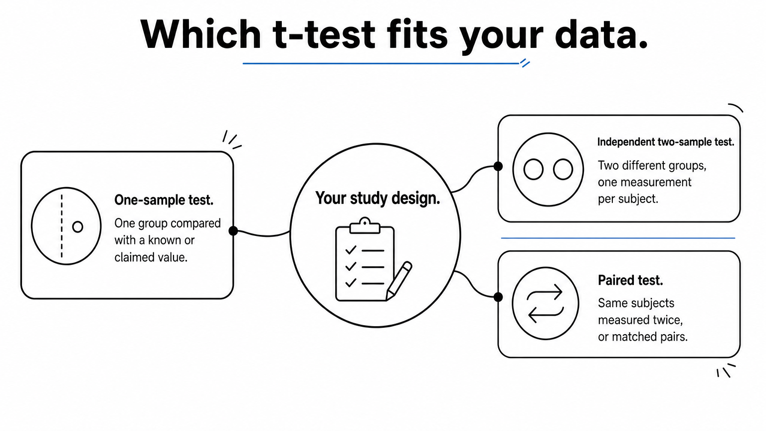
Use the one-sample formula when you have one group and a reference value, the independent formula when you have two separate groups, and the paired formula when each observation in one set has a partner in the other. The design of your study decides this, not convenience.
A quick decision table
This table maps common situations to the right version. Find the row that describes how your data were collected.
| Your situation | Version | Degrees of freedom |
|---|---|---|
| One group compared with a known or claimed value | One-sample | n − 1 |
| Two different groups, one measurement per subject | Independent two-sample (Welch by default) | Welch formula, or n1 + n2 − 2 if pooled |
| Same subjects measured twice, or matched pairs | Paired | Pairs − 1 |
Edge cases come up. Twins, matched case-control pairs and left-eye versus right-eye measurements are all paired designs, because each observation has a natural partner. Two groups of different people measured once each are independent, even if the groups are the same size.
Assumptions to check first
A t-test result is only as trustworthy as the conditions behind it. Check these before you report a p-value:
- The outcome is continuous, measured on an interval or ratio scale.
- Observations are independent, apart from the deliberate pairing in a paired test.
- The data, or for a paired test the differences, are roughly normal. This matters most below about 30 observations.
- For the pooled version, the group variances are similar. A common rule of thumb is a standard deviation ratio under 2.
Normality worries shrink as samples grow, because the sampling distribution of the mean becomes approximately normal. With small, clearly skewed samples, switch to the Wilcoxon signed-rank test for one-sample or paired data, or the Mann-Whitney U test for independent groups.
Do not use a t-test for three or more groups. Three pairwise t-tests at 0.05 give roughly a 14% chance of at least one false positive, so use ANOVA instead. Binary outcomes and proportions also need a different test.
Match the formula to how the data were collected, then confirm the assumptions, because the wrong version produces a precise-looking wrong answer.
How to read the t statistic after you calculate it
Compare the absolute value of t with the critical value for your degrees of freedom and significance level. If it is larger, p is below alpha and you reject the null hypothesis. Equivalently, convert t to a p-value and compare that with alpha.
Critical values at the 0.05 level
People often ask what t is at the 0.05 significance level. There is no single answer, because the critical value depends on degrees of freedom and on whether the test is one-tailed or two-tailed.
| df | Two-tailed t* (α = 0.05) | One-tailed t* (α = 0.05) |
|---|---|---|
| 5 | 2.571 | 2.015 |
| 10 | 2.228 | 1.812 |
| 15 | 2.131 | 1.753 |
| 20 | 2.086 | 1.725 |
| 30 | 2.042 | 1.697 |
| 60 | 2.000 | 1.671 |
| Infinite (z) | 1.960 | 1.645 |
You can compute any critical value yourself. In Excel use =T.INV.2T(0.05, df) for a two-tailed cutoff. In R use qt(0.975, df), and in Python use scipy.stats.t.ppf(0.975, df). The table also shows why t replaces z**: at low df the t cutoff is noticeably larger, which protects you from overconfidence.
What the p-value, confidence interval and effect size add
The p-value is the probability of a t at least this extreme if the null hypothesis were true. It is not the probability that the null hypothesis is true, and it says nothing about the size of the effect. A non-significant result also does not prove there is no difference. It may only mean the sample was too small.
Report a confidence interval and an effect size alongside p. The interval is the observed difference plus or minus t* times the standard error, and if it excludes the null value the result is significant at that level. Cohen's d divides the difference by a standard deviation. For our examples, d is 0.67 for the one-sample case (8 / 12), about 1.0 for the independent case (10 / √99), and 2.25 for the paired case (5.5 / 2.45). Cohen's rough benchmarks call 0.2 small, 0.5 medium and 0.8 large, but context matters more than labels.
One-tailed or two-tailed
Default to a two-tailed test, which detects a difference in either direction. Use a one-tailed test only when you decided the direction before seeing the data and a difference the other way would be meaningless to you. Software defaults vary, so check this setting every time.
Report the t statistic, degrees of freedom, p-value, confidence interval and effect size together, never the p-value alone.
Checking your t-test calculation with software
Always confirm a hand calculation with software, because one swapped formula or wrong tails setting changes the answer. Every major tool offers the three versions through a single function.
Spreadsheet, R and Python commands
Here is how each tool handles the three tests. Excel's T.TEST returns only the p-value, not the t statistic.
| Test | Excel | R | Python (SciPy) |
|---|---|---|---|
| One-sample | Compute t by hand, then =T.DIST.2T(ABS(t), df) |
t.test(x, mu = 120) |
stats.ttest_1samp(x, 120) |
| Independent, Welch | =T.TEST(A:A, B:B, 2, 3) |
t.test(x, y) |
stats.ttest_ind(x, y, equal_var=False) |
| Independent, pooled | =T.TEST(A:A, B:B, 2, 2) |
t.test(x, y, var.equal = TRUE) |
stats.ttest_ind(x, y) |
| Paired | =T.TEST(A:A, B:B, 2, 1) |
t.test(x, y, paired = TRUE) |
stats.ttest_rel(x, y) |
In R, t.test() runs Welch's version by default, while SciPy's ttest_ind pools unless you set equal_var=False. In Excel, the third argument sets tails (2 for two-tailed) and the fourth sets the type (1 paired, 2 pooled, 3 Welch).
Mistakes that change the result
Most wrong t-test results trace back to a handful of errors:
- Using the independent formula on paired data, or the reverse.
- Pooling variances when group sizes and spreads differ widely.
- Using the standard deviation where the standard error belongs, which shrinks t dramatically.
- Reading a one-tailed p-value as if it were two-tailed.
- Forgetting that Welch's df is not n1 + n2 − 2.
If your hand result and your software disagree, check the test version and the tails setting before anything else.
Running the test in PlotStudio AI
If you would rather not code these, PlotStudio AI lets you upload a CSV and ask in plain English for a Welch t-test comparing two groups. In Verification Mode you can review the plan, edit it, and approve the methods and assumptions before anything runs. You can then inspect the generated Python and export a PDF report or Jupyter notebook. Analysis runs on your machine.
Your own judgment still decides whether a t-test fits the design. Use the formulas above as a sanity check on any output. You can try it with 30 free credits and no credit card.
Using the formulas with confidence
Every t test equation is the same ratio of signal to noise. Pick the version that matches your design: one-sample for a single group against a reference value, independent for two separate groups, and paired for repeated or matched measurements. Compute the standard error, divide, work out the degrees of freedom, and compare with the critical value.
Then check the assumptions, report the confidence interval and effect size next to p, and confirm your arithmetic with software. When the data break the assumptions badly, use a rank-based alternative instead.
If you want to run these tests on your own dataset and inspect every step of the code, you can try PlotStudio AI free.