Testing of hypothesis is a statistical procedure that uses sample data to decide whether a claim about a population is believable. You start with a default claim, called the null hypothesis, usually "no effect" or "no difference". Then you calculate how surprising your data would be if that claim were true. If the data would be very surprising, you reject the claim. If they would not, you keep the claim as a possibility, without proving it.
This article covers what you need to run and read a test. You will see why it matters, the six steps of the procedure, and the vocabulary of null and alternative hypotheses, test statistics, p-values, and alpha. You will also learn how to pick among common statistical tests, follow three worked examples with full arithmetic, avoid the mistakes that sink most results, and run the calculations in code or in software.
PlotStudio AI is built for researchers who run these tests on real datasets, so the examples lean toward clinical and lab data. The logic is the same whether you work in a spreadsheet, R, Python, or an AI workspace.
Why testing of hypothesis matters for your research
Testing of hypothesis matters because every sample is noisy, and a test gives you a fixed rule for deciding whether a pattern in your data is more than chance. Without that rule, you compare averages by eye and hope you are right.
It separates a real signal from sampling noise
Draw two random samples of 20 patients from the same population and their average blood pressure will differ. Nothing changed in the population. The samples simply contain different people. Every comparison you make in a study carries this random sampling variation, and the real question is how much of the gap it can explain.

A hypothesis test answers that question with a number. It asks how likely a difference this large would be if there were truly no effect. When that likelihood is very small, chance becomes a poor explanation, and you have grounds to take the finding seriously.
It commits you to a decision rule before you see the result
The second benefit is discipline. You fix your hypotheses, your significance level, and your test before you look at outcomes. That removes the temptation to pick whichever comparison happens to look good.
It also tells a reviewer exactly what would have counted as evidence. Clinical trial protocols typically include a pre-specified statistical analysis plan for this reason. The same habit protects a graduate student's dissertation chapter.
Where it shows up, and what it cannot do
You will meet hypothesis testing wherever a decision rests on sample data:
- Clinical trials comparing a treatment group with a control group
- Epidemiology studies asking whether an exposure is linked to an outcome
- Lab experiments comparing measurements across conditions
- Surveys testing whether a proportion differs from a benchmark
- Product experiments and quality control checks
The limits matter just as much. A test does not tell you the probability that your hypothesis is true. It does not measure how large or important an effect is, and it does not prove cause. Those answers come from effect sizes, confidence intervals, and study design.
A hypothesis test tells you whether chance is a poor explanation for your data, not whether your idea is right.
How to carry out testing of a hypothesis in 6 steps
You carry out a test by stating the hypotheses, setting alpha, choosing a test, computing the test statistic, getting the p-value, and making a decision. The order matters, because the first three steps happen before you look at results.
The six steps
- State the hypotheses. Write H0 and H1 about a population parameter such as a mean, a proportion, or a difference between groups. Decide now whether H1 points in one direction or allows either.
- Set the significance level (alpha). Use 0.05 as a default. Choose 0.01 when a false positive would be costly.
- Choose the test and check its assumptions. Look at your data type, the number of groups, whether observations are independent, and whether the sample is large enough or the data roughly normal.
- Collect the data and compute the test statistic. The test statistic measures how far your sample result sits from the value H0 claims, in standard errors.
- Find the p-value or compare to the critical value. Both routes lead to the same decision.
- Decide and report. Reject H0 or fail to reject it, then report the effect size and a confidence interval alongside the p-value.
Other guides describe four, five, or seven steps. The work is the same. They merge steps one and two, or split data collection and interpretation into separate stages. If you can do the six above, you can follow any of those versions.
A worked example: one-sample t-test
Suppose a published reference puts mean resting systolic blood pressure for a patient group at 120 mmHg. You enroll 25 patients on a new care protocol. Their mean is 125 mmHg with a sample standard deviation of 10. Is the group's mean different from 120?
| Step | Work |
|---|---|
| 1. Hypotheses | H0: μ = 120. H1: μ ≠ 120 (two-sided) |
| 2. Alpha | α = 0.05, chosen in advance |
| 3. Test | One-sample t-test, because the population standard deviation is unknown. Patients are independent, and the values look roughly symmetric |
| 4. Test statistic | t = (125 − 120) / (10 / √25) = 5 / 2 = 2.5 |
| 5. P-value | With 24 degrees of freedom, the two-sided p-value is about 0.02. The critical values are ±2.064 |
| 6. Decision | 2.5 exceeds 2.064 and p < 0.05, so reject H0 |
The 95% confidence interval agrees. It runs from 125 − 2.064 × 2 to 125 + 2.064 × 2, which is about 120.9 to 129.1 mmHg. The interval excludes 120, just as the test does.
Read the result with care. The test says the group's mean is unlikely to equal 120. It does not say the protocol raised blood pressure, because you had no control group. It also cannot tell you whether a 5 mmHg difference matters clinically. That judgment belongs to you.
Six steps, in a fixed order: hypotheses, alpha, test, statistic, p-value, decision.
Key terms: hypotheses, test statistic, p-value, and alpha
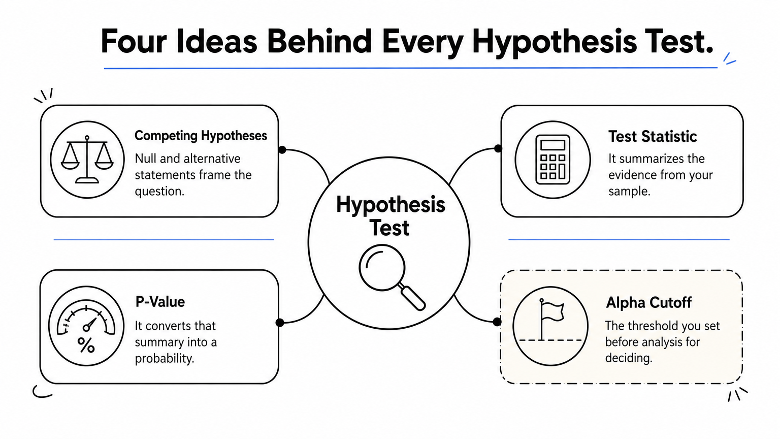
The core vocabulary of testing a statistical hypothesis comes down to four ideas. Two competing hypotheses frame the question, a test statistic summarizes the evidence, a p-value converts that summary into a probability, and alpha is the cutoff you set for deciding.
The null and alternative hypotheses
A hypothesis is a specific statement about a population, usually a numeric claim such as "the mean is 120" or "the two groups have equal means". Hypothesis testing pits two such statements against each other. The null hypothesis (H0) is the default, the status quo. The alternative hypothesis (H1 or Ha) is the claim you would conclude if the evidence is strong enough.
| Research question | H0 | H1 |
|---|---|---|
| Is the mean different from a reference? | μ = μ0 | μ ≠ μ0 |
| Is the mean higher than a reference? | μ = μ0 | μ > μ0 |
| Is the mean lower than a reference? | μ = μ0 | μ < μ0 |
| Do two groups differ? | μ1 = μ2 | μ1 ≠ μ2 |
| Is a proportion below a benchmark? | p = p0 | p < p0 |
Getting this table right is the most important part of the whole procedure. If the hypotheses do not match your research question, every later number answers a different question than the one you asked.
The test statistic and the p-value
Every test statistic has the same basic shape:
test statistic = (sample estimate − value stated by H0) / standard error
In the blood pressure example, 2.5 means the sample mean sits 2.5 standard errors above the claimed 120. A t-test, z-test, chi-square test, and F-test all follow this pattern of "observed versus expected, scaled by noise", though the formulas differ.
The p-value is the probability of getting a test statistic at least as extreme as yours, assuming H0 is true and the test's assumptions hold. A p-value of 0.02 means that if the true mean were exactly 120, you would see a result this far away in about 2% of samples. It does not mean there is a 2% chance H0 is true. That reading is the most common misinterpretation in all of statistics.
Alpha, the decision rule, and one-tailed versus two-tailed tests
Alpha is the p-value cutoff you set before analysis. The rule is simple: reject H0 when p ≤ α, otherwise fail to reject. You can reach the same decision with critical values, which mark where the rejection region begins on the test statistic's scale. For a z-test, these are the common ones:
| Alpha | One-tailed critical z | Two-tailed critical z |
|---|---|---|
| 0.10 | 1.282 | 1.645 |
| 0.05 | 1.645 | 1.960 |
| 0.01 | 2.326 | 2.576 |
A one-tailed test puts all of alpha in one direction, which gives more power in that direction and none in the other. A two-tailed test splits alpha across both tails. Pick the direction from your research question before you see the data. Choosing it afterward invalidates the stated error rate.
Alpha is a promise about your false-positive rate, so set it before the data arrive.
Type I errors, Type II errors, and statistical power
A test can go wrong in exactly two ways. A Type I error rejects a true null hypothesis, and a Type II error fails to reject a false one. Alpha controls the first. Beta and power describe the second.
The two ways a test can be wrong
You never know whether H0 is actually true, so every decision carries some risk of error. The table below shows all four outcomes.
| Your decision | H0 is true | H0 is false |
|---|---|---|
| Reject H0 | Type I error (false positive), probability α | Correct decision, probability 1 − β |
| Fail to reject H0 | Correct decision, probability 1 − α | Type II error (false negative), probability β |
Which error is worse depends on the stakes. Declaring an ineffective drug effective is a Type I error with real consequences, so you might use α = 0.01. Missing a real harm signal in a safety study is a Type II error, and you would want high power instead. For a fixed sample size, lowering alpha raises beta. You cannot push both down without more data.
What beta means and how to plan sample size
In statistics, β is the probability of a Type II error, the chance that you miss an effect that is really there. Power is 1 − β, the chance that you detect it. A common target is 80% power.
Four things raise power: a larger sample, a larger true effect, lower variability in the outcome, and a higher alpha. The first is the one you control. For comparing two group means, a rough normal-approximation formula for the sample size per group at α = 0.05 (two-sided) and 80% power is:
n ≈ 15.7 × σ² / δ²
Here σ is the outcome's standard deviation and δ is the smallest difference you care about. If σ = 10 and you want to detect δ = 5, then n ≈ 15.7 × 100 / 25, which is about 63 per group. A dedicated power calculation will add a few participants to account for the t distribution. Run this calculation before collecting data, not after a nonsignificant result.
Alpha limits false alarms, and power limits missed discoveries, so plan both before you collect data.
Statistical tests for hypothesis testing: which one to use
The right test depends on your question, your outcome type, and your design. Match those three things and the choice is usually clear.
Match the test to your question and data
| Your question | Data | Test |
|---|---|---|
| Does one mean differ from a reference value? | Numeric | One-sample t-test (z-test if σ is known) |
| Do two independent groups differ? | Numeric | Two-sample t-test (Welch version is the safer default) |
| Did the same subjects change between two time points? | Numeric, paired | Paired t-test |
| Do three or more group means differ? | Numeric | One-way ANOVA |
| Does a proportion differ from a benchmark? | Binary | One-proportion z-test |
| Are two categorical variables associated? | Counts | Chi-square test of independence |
| Are two numeric variables related? | Numeric | Test of Pearson correlation |
| Do two groups differ, with skewed or ordinal data? | Ranks | Mann-Whitney U test |
| Did paired values change, with skewed or ordinal data? | Ranks, paired | Wilcoxon signed-rank test |
| Do survival curves differ between groups? | Time to event | Log-rank test |
ANOVA deserves a note. A significant ANOVA tells you at least one group mean differs, not which one. A post hoc comparison with a multiplicity correction identifies the pair.
Z-test or t-test, and when assumptions fail
A z-test needs a known population standard deviation, which almost never happens in real research. In practice you estimate the spread from the sample, and the t-test accounts for that extra uncertainty with a slightly heavier-tailed distribution. With large samples the two give nearly identical answers, but a large n alone does not turn your analysis into a z-test.
Every test rests on assumptions, and they differ by test. Most t-tests assume independent observations and roughly normal data, or a sample large enough that the sample mean behaves normally. The classic pooled two-sample t-test also assumes equal variances, which is why Welch's version is the safer default. Chi-square tests need adequate expected counts in each cell, and one-proportion z-tests need both n·p0 and n·(1 − p0) to be at least 5.
When assumptions fail badly, a rank-based test like Mann-Whitney U is a reasonable fallback. Look at a histogram or box plot before you choose, not after.
Choose the test from your question and your data type, and check its assumptions before you trust the p-value.
More worked examples: two groups and a proportion
Two more examples show how the same six steps adapt. One compares two group means. The other tests a proportion and shows how much your choices about alpha and tails can change the conclusion.
Comparing two group means with Welch's t-test
A rehabilitation study measures a functional score after 12 weeks. The treatment group has n = 40, mean 72.4, and SD 8.0. The control group has n = 40, mean 68.0, and SD 9.0. Higher scores are better, and you have no prior reason to expect only one direction.

- Hypotheses: H0: μ1 = μ2. H1: μ1 ≠ μ2.
- Alpha: 0.05.
- Test: Welch's two-sample t-test, since the SDs differ slightly.
- Standard error: √(8.0²/40 + 9.0²/40) = √(1.6 + 2.025) = √3.625 ≈ 1.904.
- Test statistic: t = (72.4 − 68.0) / 1.904 ≈ 2.31, with about 77 degrees of freedom.
- P-value and decision: The two-sided p-value is roughly 0.02, below 0.05, so reject H0.
Now add the context. The difference is 4.4 points, and its 95% confidence interval runs from about 0.6 to 8.2. The standardized effect size (Cohen's d) is 4.4 divided by the pooled SD of about 8.5, which is roughly 0.52, a medium effect. The interval is wide, so the data are compatible with a tiny benefit and with a large one. A p-value of 0.02 hides that uncertainty, which is why you report the interval too.
A one-sided proportion test, and why alpha and tails matter
A hospital's historical 30-day readmission rate is 20%. After a discharge program, 38 of 250 patients are readmitted, so the sample proportion is 38/250 = 0.152. Did the program lower the rate?
- Hypotheses: H0: p = 0.20. H1: p < 0.20 (one-sided, because the program aims to reduce readmissions).
- Conditions: n·p0 = 50 and n·(1 − p0) = 200, both well above 5, so the normal approximation is fine.
- Standard error under H0: √(0.20 × 0.80 / 250) = √0.00064 ≈ 0.0253.
- Test statistic: z = (0.152 − 0.20) / 0.0253 ≈ −1.90.
- P-value: The one-sided p-value is about 0.029.
At α = 0.05, you reject H0. At α = 0.01, you do not. And if you had run a two-sided test, the p-value would double to about 0.058, which fails at 0.05. The same data support three different conclusions depending on choices you must make before looking. This is the strongest argument for pre-specifying alpha and the tail direction, and for reporting the exact p-value rather than only "significant" or "not significant".
The same data can pass or fail depending on alpha and tails, so fix both in advance and report the exact p-value.
Common mistakes and how to report a result
Most failed analyses fail on interpretation rather than arithmetic. Know the common mistakes, then use a fixed reporting pattern so your results are complete and checkable.
Mistakes that undermine a hypothesis test
- Saying "accept H0". A nonsignificant result means you lack evidence against H0. It does not show H0 is true, especially with a small sample and low power.
- Switching the tail after the fact. Moving to a one-sided test because the data leaned one way inflates your false-positive rate.
- Running many tests and reporting the winners. Each extra test is another chance for a false positive. At α = 0.05, 20 independent tests of true nulls produce about one false positive on average. Pre-specify your primary outcome or apply a multiplicity correction.
- Ignoring dependence. Repeated measures on the same patient are not independent. Treating them as independent makes p-values too small.
- Equating significance with importance. With a huge sample, a trivial difference becomes significant. With a tiny sample, a large difference may not. Always look at the effect size.
- Stopping data collection when p dips below 0.05. Peeking and stopping early breaks the error guarantees unless the design planned for it.
A reporting template you can adapt
A good results sentence names the test, the estimate, the uncertainty, and the p-value. Copy this structure and fill in your numbers:
We compared [outcome] between [group A] and [group B] using a [test name]
with a two-sided significance level of 0.05, specified before data collection.
[Group A] (mean = __, SD = __, n = __) differed from [Group B]
(mean = __, SD = __, n = __) by __ (95% CI __ to __), t(__) = __, p = __,
Cohen's d = __. [State how you checked assumptions, and any deviations.]
Notice what the template forces. It makes you state the effect with its interval, name the test, and record that alpha was fixed in advance. A reader can then judge your result without guessing what you did.
Report the estimate, its confidence interval, and the exact p-value, because "p < 0.05" alone is not a result.
Running a hypothesis test in Python or PlotStudio AI
You can run any of these tests in a few lines of Python, or in an AI workspace that writes and runs the code for you. Either way, the test choice and the interpretation stay your responsibility.
Hypothesis tests in Python with SciPy
SciPy's stats module covers the tests from the table above. The snippet below reproduces both worked examples from summary statistics, so you can check your own arithmetic.
import math
from scipy import stats

# One-sample t-test from summary statistics (blood pressure example)
xbar, mu0, s, n = 125, 120, 10, 25
t_stat = (xbar - mu0) / (s / math.sqrt(n))
p_value = 2 * stats.t.sf(abs(t_stat), df=n - 1)
print(round(t_stat, 2), round(p_value, 3))   # t = 2.5, p near 0.02

# Welch two-sample t-test from summary statistics (rehabilitation example)
res = stats.ttest_ind_from_stats(72.4, 8.0, 40, 68.0, 9.0, 40, equal_var=False)
print(round(res.statistic, 2), round(res.pvalue, 3))   # t = 2.31, p near 0.02
With raw data in arrays, these functions do the work directly:
| Test | SciPy function |
|---|---|
| One-sample t-test | stats.ttest_1samp(data, popmean=120) |
| Two-sample t-test (Welch) | stats.ttest_ind(a, b, equal_var=False) |
| Paired t-test | stats.ttest_rel(before, after) |
| One-way ANOVA | stats.f_oneway(g1, g2, g3) |
| Chi-square test of independence | stats.chi2_contingency(table) |
| Mann-Whitney U | stats.mannwhitneyu(a, b) |
| Wilcoxon signed-rank | stats.wilcoxon(before, after) |
| Kruskal-Wallis | stats.kruskal(g1, g2, g3) |
Using an AI workspace without giving up control
If you do not code, or you want to skip repetitive scripting, PlotStudio AI runs this workflow from plain-English questions. You upload a dataset and ask something like "Does the treatment group score differ from controls?". Specialized agents then plan the analysis, write and execute Python, and return the figures, test results, and interpretation on a saved analysis page.
The part that matters for rigor is Verification Mode. It lets you review the proposed plan, question it, and edit the statistical methods and assumptions before anything runs. You can also inspect the generated code and export the work as a Jupyter notebook or a PDF report, so every step is checkable. Analysis runs on your own machine. If your data are clinical or otherwise regulated, still confirm your institution's privacy and ethics requirements.
PlotStudio is an assistant, not a substitute for judgment. You still decide the hypotheses, alpha, and tail direction, and you still check assumptions. It is free to try with no credit card.
Whether you write the code or an assistant does, you own the hypotheses, the test choice, and the interpretation.
Putting hypothesis testing to work
Testing of hypothesis is a disciplined way to ask whether your data are surprising under a default claim. You state H0 and H1, fix alpha, pick a test that fits your question and data, compute the test statistic and p-value, and decide. The decision is "reject" or "fail to reject", never "proven".
The calculation is the easy part. The value comes from the choices around it: the right hypotheses, an honest alpha and tail direction, adequate power, assumption checks, and a report that includes effect sizes and confidence intervals. Do those well and your p-value means what you think it means.
To practice on your own data, upload a dataset and walk through a test from question to report. You can try PlotStudio AI free and inspect the plan, code, and results for every step.