The best way to learn sample hypothesis testing is to follow complete worked examples, and the six below cover most problems you will meet: a one-sample t-test, a two-sample t-test, a paired t-test, a one-proportion z-test, a chi-square test, and a one-way ANOVA. A good example states both hypotheses, shows every number, and ends with a plain-language conclusion. Pick the example that matches your data. Use the first if you compare one mean to a target, and the second or third if you compare two groups or two time points. The fourth and fifth are for rates and category counts, and the sixth is for three or more groups.
Most people do not struggle with the arithmetic. They struggle to know which test fits, what the null hypothesis should say, and how far a p-value lets them go. A textbook formula does not settle those questions. A solved problem does.
Every example here follows the same five steps: state the hypotheses, set alpha, choose the test, compute the statistic and p-value, and decide. We build PlotStudio AI, a research analysis workspace where you can request these tests in plain English and inspect the Python behind them, so we care about getting the setup right. The numbers below are small and invented for teaching, which means you can verify each one by hand.
1. One-sample t-test: a battery life claim
A one-sample t-test checks whether a sample mean differs from a claimed value when you do not know the population standard deviation. This example also shows why the choice of tail matters.

The setup
A manufacturer claims its laptop battery lasts at least 10 hours. You test 16 batteries and get a mean of 9.4 hours with a sample standard deviation of 1.2 hours.
- H0: μ ≥ 10 hours
- H1: μ < 10 hours
- Test: left-tailed one-sample t-test, because the population SD is unknown
- Alpha: 0.05
The calculation
The standard error is 1.2 / √16 = 0.30. The test statistic is then t = (9.4 − 10) / 0.30 = −2.00.
- Degrees of freedom: 16 − 1 = 15
- Critical value at alpha 0.05, left tail: −1.753
- Left-tail p-value: about 0.032
How to read the result
Because −2.00 falls beyond −1.753 and 0.032 is below 0.05, you reject H0. The sample gives evidence that the true mean battery life is below 10 hours.
Now switch to a two-sided test on the same data. The p-value doubles to about 0.064, and you would fail to reject H0. Choose the tail from the research question before you look at the data, never after.
The same data can pass or fail depending on the tail, so fix the direction before you see the results.
2. Two-sample t-test: comparing two teaching methods
A two-sample t-test compares the means of two independent groups. Use Welch's version unless you have a strong reason to assume equal variances.
The setup
Two different groups of 25 students learn the same unit, one with Method A and one with Method B. Method A has a mean score of 82 (SD 8). Method B has a mean of 77 (SD 9).
- H0: μA − μB = 0
- H1: μA − μB ≠ 0
- Test: two-sided Welch t-test
- Alpha: 0.05
The calculation
The standard error of the difference is √(8²/25 + 9²/25) = √5.80 = 2.41. That gives t = 5 / 2.41 = 2.08.
- Welch degrees of freedom: about 47
- Two-sided p-value: about 0.043
- 95% confidence interval for the difference: about 0.2 to 9.8 points
How to read the result
You reject H0 at 0.05, since 0.043 is below it. Method A's mean is higher by 5 points, and the data are hard to square with no difference.
Look at the interval before you celebrate, though. It barely excludes zero, and the effect size (Cohen's d, about 0.59) is moderate. If students chose their own method, a lurking factor could explain the gap, so only random assignment supports a causal claim.
A p-value just under 0.05 is a prompt to read the confidence interval, not a verdict.
3. Paired t-test: blood pressure before and after
A paired t-test compares two measurements on the same subjects, so you test the mean of the differences instead of two separate means.

The setup
Nine patients have their systolic blood pressure measured before and after an eight-week program. The differences (after minus before) have a mean of −6.0 mmHg and an SD of 6.0 mmHg.
- H0: μd = 0
- H1: μd ≠ 0
- Test: two-sided paired t-test
- Alpha: 0.05
The calculation
The standard error is 6.0 / √9 = 2.0. The statistic is t = −6.0 / 2.0 = −3.00, with 8 degrees of freedom.
- Two-sided p-value: about 0.017
- Critical value: ±2.306
- 95% confidence interval for the mean change: −10.6 to −1.4 mmHg
How to read the result
You reject H0. Average blood pressure fell by about 6 mmHg, and the interval stays below zero. Pairing the data matters here. Treating the before and after readings as two independent groups would ignore that the same people appear in both, and it would throw away statistical power.
This design has no control group. Placebo effects and regression to the mean could produce part of the drop, so the test shows that blood pressure changed, not that the program caused it.
Pair the data when the subjects are the same, and remember that a change over time is not proof of cause.
4. One-proportion z-test: a treatment completion rate
A one-proportion z-test compares an observed proportion with a known or claimed rate. This example ends without rejecting H0, which is a result you will see often.
The setup
A clinic's follow-up program has a long-run completion rate of 60%. After adding a reminder system, 130 of 200 patients complete it, which is 65%.
- H0: p = 0.60
- H1: p ≠ 0.60
- Test: two-sided one-proportion z-test
- Alpha: 0.05
Check the conditions first. Both np0 = 120 and n(1 − p0) = 80 are at least 10, so the normal approximation is fine.
The calculation
Under H0, the standard error uses the claimed rate, not the observed one: √(0.60 × 0.40 / 200) = 0.0346. Then z = (0.65 − 0.60) / 0.0346 = 1.44.
- Critical values: ±1.96
- Two-sided p-value: about 0.15
How to read the result
Since 1.44 is inside ±1.96 and 0.15 exceeds 0.05, you fail to reject H0. The 5-point gain is compatible with ordinary sampling variation.
That does not show the reminders do nothing. With 200 patients, this test has little power to detect a 5-point improvement. A larger sample, or a pre-registered target effect size, would give a firmer answer.
Failing to reject H0 means the evidence is insufficient, not that the null hypothesis is true.
5. Chi-square test: treatment and outcome
A chi-square test of independence asks whether two categorical variables are associated, using counts instead of means.
The setup
You randomly assign 200 patients to Drug A or Drug B and record whether each improved.
| Improved | Not improved | Total | |
|---|---|---|---|
| Drug A | 60 | 40 | 100 |
| Drug B | 45 | 55 | 100 |
| Total | 105 | 95 | 200 |
H0 says outcome is independent of the drug. H1 says they are associated. Alpha is 0.05.
The calculation
Each expected count is row total × column total / 200. For both drugs, that is 52.5 improved and 47.5 not improved. Then χ² adds (O − E)² / E over the four cells: 1.07 + 1.18 + 1.07 + 1.18 = 4.51.
- Degrees of freedom: (2 − 1)(2 − 1) = 1
- Critical value at 0.05: 3.84
- p-value: about 0.034
How to read the result
You reject H0. Improvement was 60% on Drug A and 45% on Drug B, so the outcome is associated with the drug. The test itself gives no direction, so compare the row percentages to say which drug did better.
Many software packages apply a continuity correction to 2 × 2 tables. Here it gives χ² = 3.93 and p ≈ 0.047. The decision holds, but it is much closer, so state which version you used.
Chi-square flags an association, and the row percentages tell you what that association looks like.
6. One-way ANOVA: three fertilizers
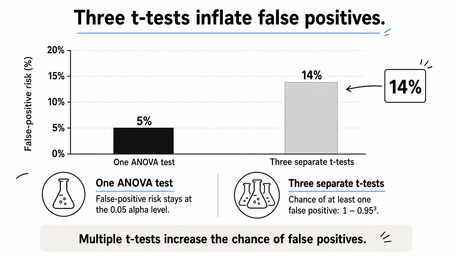
One-way ANOVA tests whether three or more group means are all equal. It avoids the inflated false-positive risk of running many t-tests.
The setup
You measure plant growth in centimeters after four weeks under three fertilizers, with five plants each.
| Fertilizer | Growth (cm) | Mean |
|---|---|---|
| A | 5, 6, 7, 6, 6 | 6 |
| B | 7, 8, 8, 9, 8 | 8 |
| C | 6, 7, 7, 8, 7 | 7 |
H0: μA = μB = μC. H1: at least one mean differs. Alpha is 0.05.
The calculation
The grand mean is 7. Between groups, SSB = 5 × (1 + 1 + 0) = 10 with 2 degrees of freedom, so MSB = 5. Within groups, each fertilizer contributes 2, so SSW = 6 with 12 degrees of freedom and MSW = 0.5.
- F = MSB / MSW = 10.0
- Critical F(2, 12) at 0.05: 3.89
- p-value: about 0.003
How to read the result
You reject H0, so at least one fertilizer produces a different mean growth. ANOVA does not say which one. Follow up with a post hoc test such as Tukey's HSD to compare pairs.
Skipping ANOVA and running three separate t-tests at 0.05 raises the chance of at least one false positive to about 14% (1 − 0.95³). Check independence, roughly normal residuals, and similar spread across groups. If those fail, a Kruskal-Wallis test is the usual fallback.
A significant F tells you that the means differ somewhere, and a post hoc test tells you where.
Which test fits your own data
Choose the test from the type of data and the number of groups you compare. The table maps each question to the example above.
Match the question to the test
| Your question | Data | Test | Example |
|---|---|---|---|
| Does one mean differ from a target? | One numeric sample | One-sample t | 1 |
| Do two separate groups differ in mean? | Numeric, two groups | Welch t | 2 |
| Did the same subjects change? | Paired numeric | Paired t | 3 |
| Does a rate differ from a known rate? | One yes/no outcome | One-proportion z | 4 |
| Are two categories associated? | Counts in a table | Chi-square | 5 |
| Do three or more means differ? | Numeric, 3+ groups | One-way ANOVA | 6 |
If your data break a test's assumptions, such as heavy skew with small samples, a nonparametric alternative like the Mann-Whitney U test is the next step.
Mistakes that sink a hypothesis test
Most wrong conclusions come from the same few habits:
- Picking one-tailed or two-tailed after seeing the result
- Reading a high p-value as proof that H0 is true
- Reporting a p-value without an effect size or confidence interval
- Treating paired measurements as independent groups
- Running many tests and reporting only the significant ones
Decide the hypotheses, the tail, and alpha first, then let the data speak.
Pick the test, then follow the same steps
Every example above ran on the same logic: write H0 and H1, fix alpha, choose a test that fits the data, compute the statistic and p-value, and state the conclusion in plain words. The test changes with your data, but the reasoning does not. Report the effect size and confidence interval next to every p-value.
When you are ready to run these tests on a real dataset, you can try PlotStudio AI free. The free trial includes 30 credits and needs no credit card. You can review the proposed analysis plan before it runs and inspect the generated code, while the final judgment on your methods stays with you.